Appearance

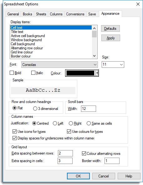
These options let you customize the appearance of the spreadsheet, for example, the fonts and colours used for different spreadsheet attributes.

To access this dialog select Tools | Spreadsheet Options then click the Appearance tab.
Set options as required. (For example, select Cell text from the Display items list then select a font from the Font dropdown list to change the cell text font.)
Click Apply to apply your changes.
This will update any displayed spreadsheet without closing the dialog, so that you can see the visual effect of any changes.
When you have finished making changes click OK to close the dialog.

Display items	You can customize the font and colour of all items in this list.
Defaults	Resets all options on this tab to their default values. Settings on other tabs remain unchanged.
Apply	Apply your changes but keep the dialog open so you can make more changes as required.
Font	Select a font from the dropdown list to apply to whichever item you have selected in the Display items list.
Size	Select the size of your chosen font from the dropdown list. The sizes in the Size list depend on the selected font.
Bold	Lets you apply bold to your chosen font.
Italic	Lets you apply italic to your chosen font.
Colour	Select a colour from the dropdown list to apply to whichever item you have selected in the Display items list. If you want to select a colour that is not in the list, click the dropdown arrow then click Custom. This opens the colour palette, which lets you choose from a wider range of colours.
Row and column headings	This controls the visual appearance of the row and column headings. Flat – Gives the headers a flat appearance. 3 dimensional – Gives the headers a 3D appearance.
Scroll bars width	Lets you set the width of the scroll bars. Making this too small will make the bottom left frame buttons. We recommend values between 10 and 16.
Column names justification	This controls the position of the column names, which can be centre justified, left justified, right justified or use the same justification as the cells in the column.
Use icons for types	Select this to include icons in the column names to distinguish between data types (variate, text or factor). A factor is indicated by a red exclamation mark at the start of the column name. A text is indicated by a green at the start of the column name.
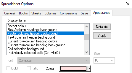
Use colours for types	When selected, the background colour of the column name header distinguishes the data type (variate, text or factor). The background colour of factor and text column headers are set in the Display items list: Factor columns header background and Text columns header background.
Display spaces for underscores within column names	When selected, underscores in column names are displayed as spaces. This is ignored for underscores at the start and end of a name. Note: column names with a leading underscore will not display in the Data View. Column _C1 is not displayed in the Data View on the left
Grid layout	Lets you control the appearance of the spreadsheet’s grid. Extra spacing between rows – Lets you control the height of the rows, by specifying the vertical cell padding added between the cell text and the grid lines above or below it. A value of -1 or -2 can be used to minimize the white space above and below the text. Extra spacing in cells – Lets you specify the cell padding, which separates the displayed cell text from the left or right grid line (depending on the column justification). This must not be a negative number. Colour alternative rows – Applies background colour to the alternating rows in the spreadsheet. The background colour of the cells and alternating rows are set by Cell background and Alternating row colour in the Display items list. Border width – Lets you specify the width of the grid’s border. This must be a positive number.

Updated on March 1, 2019

Was this article helpful?

Yes No