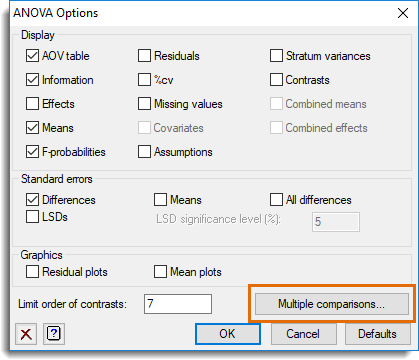
Multiple Comparisons is available via the ANOVA Options dialog, but only if the option Show multiple comparisons on menus has been enabled on the Tools | Options | Menus tab.
Multiple comparison tests are designed to take account of the fact that there may be many possible comparisons between pairs of treatment means in an analysis of variance (with n treatments there are n (n-1) / 2). So, some researchers feel that their significance levels should be adjusted to take account of all the tests that they might make – and this can be achieved by use of a multiple comparison test.
Conversely, it has been pointed out that multiple comparisons are unnecessary if you have only a small number of comparisons to make – either because there are few treatments, or because you should have identified beforehand the comparisons that you feel are likely to be of interest. Also, they are inappropriate if the treatments have any sort of structure. For example, the levels of a treatment factor may represent different amounts of a substance like a fertiliser or a drug. It would then be more sensible to assess the treatment effect over all its levels by fitting some sort of trend (see ANOVA Contrasts), and implausible to assume that only some of the amounts might have an effect. Alternatively, the treatments may have a factorial structure, and you should then be more interested in studying the main effects and interactions of the various factors. For further discussion of the issues see Nelder (1971), Maindonald and Cox (1984) and Perry (1986).
The methodology implemented here closely follows that described in Chapter 5 of Hsu (1996). You can also use this method to calculate a set of simultaneous confidence intervals i.e. intervals whose formation takes account of the number of intervals formed and the fact that the intervals are (slightly) correlated because of the use of a common variance (see Hsu 1996 and Bechhofer, Santner and Goldsman 1995). The methodology implemented in the procedure closely follows that described in Section 1.3 of Hsu (1996).
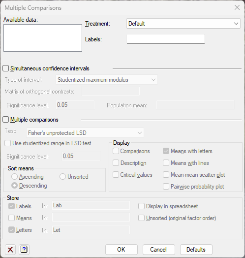
Available data
This lists data structures appropriate to the current input field. The contents will change as you move from one field to the next. Double-click a name to copy it to the current input field or type the name.
Treatment
Lists the treatment factors for the current analysis. Select the treatment factor that the multiple comparisons and/or simultaneous confidence intervals are to be performed on. If no treatment factors have been specified in the current model then the list will include Default. Select this to form the multiple comparisons and simultaneous confidence intervals using the first treatment factor that appears in the subsequent ANOVA model formula.
Labels
Specifies labels for the means.
Simultaneous confidence intervals
If selected, this enables options which can be used to specify simultaneous confidence intervals. This option is unavailable for unbalanced ANOVA.
Type of Interval
This lists the different types of interval that can be formed. The method Individual calculates the intervals as if they were independent, each with the input probability. Studentized maximum modulus calculates the intervals as correlated, each with a probability adjusted for the multiplicity of intervals. The two settings Inequality and Bonferroni calculate the intervals as independent, but with a probability adjusted for the multiplicity of intervals. These produce very similar intervals although the Bonferroni intervals are always slightly larger. Scheffé calculates the intervals using pivoted F statistics. Refer to Hsu (1996, Section 1.3.7) for details of this last setting. The method Dunnett is for forming simultaneous confidence intervals around a control. The default is Studentized maximum modulus because this produces exact simultaneous confidence intervals.
Matrix of orthogonal contrasts
Specifies a matrix defining contrasts amongst the means to be used when forming confidence limits. Each row of the matrix contains a contrast similar to the specification for Regression contrasts in Analysis of Variance but, unlike the Regression contrasts, the contrasts must all be orthogonal. This option is not available for Dunnett’s test.
Control level for comparison (Dunnett’s test only)
For Dunnett’s test this specifies which of the means of the terms is the control. This can be a comma separated list of scalars to identify the levels of the factors that correspond to the control, or strings to identify the level of any factor that has labels. If you supply labels you must enclose them within quotes. For example, ‘A’,’B’. If this field is left blank then the reference level of the factors is used.
Significance level
Specifies the experiment-wise significance level for the intervals. You must enter a number between 0 and 1 (Default 0.05).
Population mean
Lets you specify a (population) mean to be tested for inclusion in each interval. This option is not available for Dunnett’s test.
Multiple comparisons
If selected, this enables options which can be used to specify multiple comparisons.
Test
This lets you select the type of multiple comparison tests to be performed. The following choices are available:
- Tukey
- Student-Newman-Keuls
- Ryan/Einot-Gabriel/Welsch multiple range
- Duncan
- Scheffé
- Fisher’s protected LSD
- Fisher’s unprotected LSD
- Bonferroni
- Sidak
Please see the references below for a full technical description of the methods used when calculating these statistics. Only the last three methods are available for an unbalanced ANOVA.
Use studentized range test in LSD test
If the Fisher’s Protected Least Significant Difference or the Fisher’s Unprotected Least Significant Difference test are selected, the LSD test uses the Studentized Range statistic rather than Student’s t (for further information see Hsu, 1996, page 139).
Sort means
Lets you arrange the means in either Ascending or Descending order.
Significance level
Specifies the experiment-wise significance level for the intervals. You must enter a number between 0 and 1 (Default 0.05).
Display
Specifies which items of output are to be produced.
| Comparisons | The differences between the pair of means, upper and lower confidence limits for the differences, t-statistics and an indication of whether or not they are significant. |
| Description | Description including information such as the experiment-wise and compartment-wise error rates. |
| Critical values | Gives critical values for the t-statistic for situations where these do not vary amongst the comparisons (i.e. for the Scheffe, Bonferroni and Sidak methods, as well as the Fisher LSD methods, provided all the comparisons have the same number of residual degrees of freedom). |
| Pairwise probability plot | The probabilities of differences between means displayed in a shade plot. |
| Means with letters | The means, with identical letters (a, b etc.) alongside those that do not differ significantly. |
| Means with lines | The means, with lines joining those that do not differ significantly. |
| Mean-mean scatter plot | Produces a mean-mean scatter plot (see Hsu 1996, pages 151-153). |
Store
Specifies which items of output are to be saved.
- After selecting the appropriate boxes, type the names for the identifiers of the data structures into the corresponding In: fields.
The results will be in the order specified in the Sort means option, unless the Unsorted option is selected.
| Labels | The labels for the predicted means. |
| Means | The predicted mean values. |
| Letters | Letters indicating which means are significantly different. |
Display in spreadsheet
The saved results will also be displayed within a new spreadsheet window.
Unsorted (original factor order)
The saved results will also be displayed in order of the original factors. Using this option allows multiple saved sets of results from different y-variates to be combined into a single spreadsheet later.
References
- Bechhofer, R.E., Santner, T.J. and Goldsman, D.M. (1995). Design and Analysis of Experiments for Statistical Selection, Screening, and Multiple Comparisons. Wiley, New York.
- Hsu, J.C. (1996). Multiple Comparisons Theory and Methods. Chapman & Hall, London.
- Maindonald, J.H. and Cox, N.R. (1984). Use of statistical evidence in some recent issues of DSIR agricultural journals. New Zealand Journal of Agricultural Research 27, 597-610.
- Nelder, J.A. (1976). Discussion on papers by Wynn, Bloomfield, O’Neill and Wetherall. Journal of the Royal Statistical Society, Series B 33, 244-246.
- Perry, J.N. (1986). Multiple-comparison procedures: a dissenting view. J. Econ. Entomol. 79, 1149-1155.
- Family-wise error rate. https://en.wikipedia.org/wiki/Family-wise_error_rate
- Tukey’s range test. https://en.wikipedia.org/wiki/Tukey%27s_range_test
- Student-Newman-Keuls method. https://en.wikipedia.org/wiki/Newman%E2%80%93Keuls_method
- Duncan’s new multiple range test. https://en.wikipedia.org/wiki/Duncan%27s_new_multiple_range_test
- Scheffé’s method. https://en.wikipedia.org/wiki/Scheff%C3%A9%27s_method
- Bonferroni correction. https://en.wikipedia.org/wiki/Bonferroni_correction
- Šidák correction. https://en.wikipedia.org/wiki/%C5%A0id%C3%A1k_correction
See also
- ANOVA Contrasts for specifying polynomial and regression contrasts
- Multiple Comparisons for REML dialog.
- Multiple Comparisons for Predictions dialog in regression menus.
- AMCOMPARISON procedure for all pairwise multiple comparison tests
- CONFIDENCE procedure for forming simultaneous confidence intervals
- AMDUNNETT procedure for forming simultaneous confidence intervals around a control