Conditional formatting lets you colour numeric cells within a column according to a set of conditional rules. Up to three rules can be applied to a column, although the between rule counts as two. Rules are applied sequentially, so if a cell matches the rule 1, rules 2 and 3 will be ignored. Thus the ordering of rules can be important. For example the rules Greater than 10, Greater than 20 and Greater than 30 in that order would not give the required three colours, as all values greater than 20 or 30 meet the first condition and so would just be coloured in the first specified colour. To get three colours the rules would need to be in the order of the most restrictive to the least, i.e. Greater than 30, Greater than 20 and Greater than 10.
The middle image below shows a spreadsheet that records the pulse rates of patients. Conditional formatting has been applied to two of the columns: Pulse1 and Pulse2.
The image on the left shows the formatting applied to column Pulse1: high value cells are coloured magenta and low value cells are coloured light blue by matching one of two conditions:
- Greater than or equals
- Less than or equals.
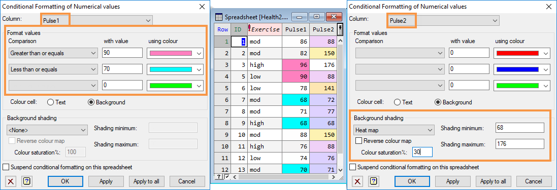
The image on the right shows that we’ve applied a different set of formatting options to column Pulse2: high values take on yellow hues while low values are coloured in shades of purple. Graduated colours have been applied by selecting Heat Map for the Background shading while Colour saturation is reduced to 30% to make the colours less bright.
You can set all columns to use the same conditions and colour scheme, or apply rules and colours on a per-column basis as shown above.
If you want to use the same conditional colouring rules across several columns, select the columns first.
- From the menu select Spread | Column | Conditional Formatting.
- Select a column from the dropdown list.
- If you pre-selected columns in the spreadsheet before opening this dialog the option All Selected Columns will be available to apply conditional colouring to all selected columns.
- All Numerical Columns lets you apply conditional colouring to all numerical columns.
- EITHER
In the Format values section, set conditions and associated colours as required. - Choose whether to apply the conditional colours to the Text or cell Background.
OR - Leave the Format values section blank and select a Background shading option from the dropdown list (see table further down the page for a full description of each option).
- Set other options as required then click Apply to test your colour scheme and leave the dialog open (so you can tweak the settings) or click OK to set the colours and close the dialog.
You can combine Format values and Background shading within a column e.g. you can apply a red colour to every cell with a high value, and apply a heat map to all other values.
| Comparison | Lists the available conditions for conditional colouring. Leave this blank if you want to use one of the pre-defined Background shading options such as Heat map or Outlier map. |
| With value | Enter a number to compare column values with. If the comparison is true the selected colour will be applied. |
| Using colour | Select a colour to use when the conditional statement is true. |
| Colour cell | This controls whether conditional colouring is applied to cell text or the cell background. |
| Background shading |
Lets you apply a pre-defined colour scheme to your column cells. Each scheme provides a range of colours that are graduated between the Shading minimum and Shading maximum values (these values are taken from the lowest and highest values in the selected spreadsheet column).
|
| Shading minimum | The minimum value used in the colour shading. Values close to, or below the minimum value will be given the first colour in the colour map. |
| Shading maximum | The maximum value used in the colour shading. Values close to, or above the maximum value will be given the last colour in the colour map. |
| Reverse colour map | Select this to reverse the colour list. For example, the Blue-Red map will go from red for the minimum to blue for the maximum. |
| Colour saturation % | This controls the intensity of the colours. A value of 100% gives the maximum intensity with bright colours, while lower percentages give lighter pastel colours. |
| Suspend conditional formatting on this spreadsheet | Select this to suspend conditional formatting on all columns. This let you turn off colours temporarily, while retaining the ability to re-enable them later. |
| Apply | Apply your settings but keep the dialog open. |
| Apply to all | Apply your settings to all columns in the spreadsheet and close the dialog. |