Opening an Excel file using the import wizard involves a number of steps. You can can perform a simple import by working through steps one and two (detailed below) then clicking Finish, or complete all steps, which lets you filter out non-required data and convert or manipulate the remaining data before displaying it in a Genstat spreadsheet.
- From the menu select Spread | New | Excel Import Wizard.
- Navigate to your file then select it and click Open.
This dialog shows you a preview of all the worksheets (prefixed with S:) and named ranges (prefixed with R:) in the Excel spreadsheet. If you have any named ranges in the file then these have the advantage that both the sheet and cell range are specified permanently in the Excel file. These are automatically updated if further rows or columns are inserted into the cell range.
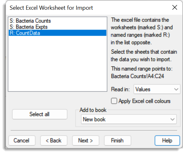
- Select the required worksheets or ranges. You can select multiple items by holding down Ctrl while clicking items with the mouse, or click the Select all button to import everything. If two or more worksheets or named ranges are selected then the wizard goes straight to step 5 and all the data are opened into a multi-paged book. If multiple data ranges are to be loaded from the same worksheet, then the import wizard will to be used multiple times on the same file specifying the range of cells each time.
-
The Read in option lets you select what cell data to read in from Excel such as the data values, cell formulae or font names. See our video on using the Read in options for examples of usage.
- The Apply Excel cell colours option displays the Excel cell and font colours in the resulting Genstat spreadsheet. Note: applying Excel colours to large spreadsheets can use a large amount of extra memory.
- The Add to Book dropdown list contains the names of any workbooks you have open in Genstat: if you have no workbooks open it will only contain New Book.
-
- Use Add to Book to select your open workbook or select New Book to create a new one, then click Next to move to step three or Finish to skip to step 6.
| Values | The normal cell values displayed in Excel |
| Formulae | The formulae as text used in the cells |
| Font colours | The font or foreground colour used in the cells |
| Cell colours | The cell or background colour used in the cells |
| Font names | The font names used in the cells |
| Styles | The font styles (bold, italic, underline) as an integer used in the cells |
| Font size | The font size as a number used in the cells |
The colours are in Genstat RGB numerical format (=256*(256*red + green) + blue, where red, green and blue can take values 0…255) for colours, the style is composed as bold + 2*italic+ 4*underline where bold = 1 if the font is bold and 0 otherwise, italic = 1 if the font is italic and 0 otherwise, and underline = 1 if underlined, 2 if double underlined, 3 if single accounting underlined,4 if double accounting underlined and 0 otherwise. Sometimes users encode data in the cell formats, for example colouring odd values, and this facility allows this information to be recovered and used in an analysis. The reading of the formulae also allows you to check for consistency in these.
This dialog provides a preview of the data in the selected worksheet. The data are truncated to display 8 characters per cell and the first 20 columns and 20 rows of the data rectangle.
- To specify a range of cells select Specified Range then type the start and finish cells names separated by a colon, e.g. A1:E13.
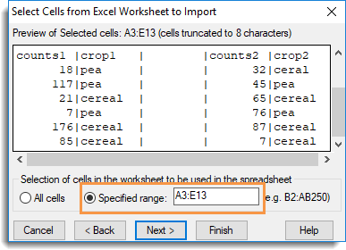
- Click Next to move to step four or Finish to skip to step 6.
This dialog provides a preview of the columns in the selected worksheet or range. Only columns displayed in the Selected columns list will be imported. All columns will be selected by default.
- To import all columns click Next to move to step five or Finish to skip to step 6. If you want to select columns to import continue reading below.
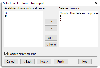
- To remove columns from the list double-click them to move them back into Available columns within cell range.
You can select multiple columns by holding down Ctrl while clicking with the mouse, then click
 to move them back across in one action.
 - To remove empty columns ensure Remove empty columns is selected. Deselect this option if you want to import empty columns.
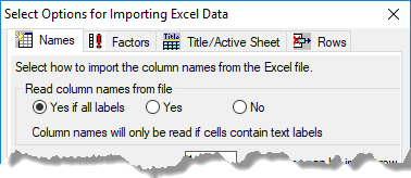
This step lets you specify the layout of the data within the worksheet or named range. These options are separated on 4 different tabs.
- To accept the defaults click Finish to import the file.
OR
Set options as required by clicking each tab in turn then click Finish.
The options on each tab are explained at the bottom of this page.
When you click Finish Genstat will read the data from the Excel file and close the wizard. At this point your new spreadsheet should open and display the imported data. However, as part of the import process Genstat will look at your data columns and if it detects a high proportion of repeated values it will prompt you to convert those columns to factors. Similarly, if there are missing values in a factor column in your source file, you will be prompted to auto-fill these.
Converting data columns to factors
Genstat will prompt you to convert columns to factors when the column contains x number of repeated values. You can set the number of repeated values in Tools | Spreadsheet Options then click the Conversions tab. Select Suggest converting columns with <=x unique items to factors and set the number as required.
- Double-click a column name to convert it to a factor. This action puts an F: at the beginning of the column name.
- When you select a column to convert the Factor button changes to Leave. This allows you to deselect a column if you make a mistake.
- Convert all selects all columns to be converted, while Leave all will undo all selections i.e. no columns will be converted.
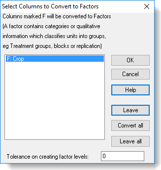
- Make your selections then click OK.
Filling empty factor cells
If you designated any of your columns as factors (by appending an exclamation mark ![]() to the column name in the source file) AND these columns contain a high proportion of missing values, you will be prompted to automatically fill the empty factor cells. It is common to put patterned data in with blanks below values in spreadsheets, as shown in the image below.
to the column name in the source file) AND these columns contain a high proportion of missing values, you will be prompted to automatically fill the empty factor cells. It is common to put patterned data in with blanks below values in spreadsheets, as shown in the image below.
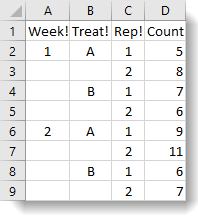
In the first column, the missing values below 1 are understood to be 1s but have not been entered. People commonly create tables like this, but you need the full data with all 1, 2, A and Bs filled in for data analysis.
- Double-click a column name to fill in any missing values. This action puts an F: at the beginning of the column name.
- When you select a column to fill the Fill button changes to Leave. This allows you to deselect a column if you make a mistake.
- Fill all selects all columns to be filled, while Leave all will undo all selections i.e. no columns will be converted.
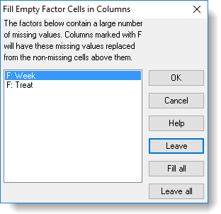
- Make your selections then click OK.
Options
These options specify the layout of column names.
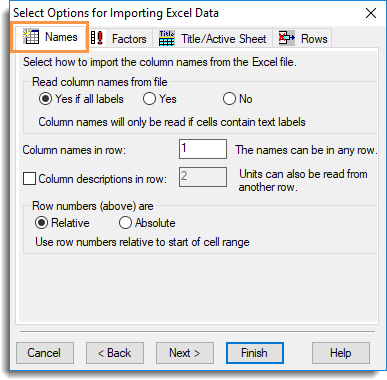
| Read column names from file | Controls whether the imported column names are used. Yes if all labels – Read the column names from the row specified in the Column names in row option if all the cells in this row contain labels only or are empty. A default column name will be generated for an empty cell. Yes – Use the cells specified in the Column names in row option . If a cell contains a number, then it will be prefixed with “_” to ensure it is a valid Genstat identifier name. No – Generate default names for the columns, ignoring those in the file. |
| Column names in row | Specifies the row number to use for column names. |
| Column descriptions in row | When selected, the cells in the specified row number will be used for column descriptions. |
| numbers (above) are | Controls whether the row numbers are relative to the data range or relate to a whole worksheet. Relative – Row numbers start from the top of the restricted cell range. Absolute – Row numbers start from the top of the worksheet and thus correspond to the absolute row numbering in the file. |
These options control if and how columns are converted to factors.
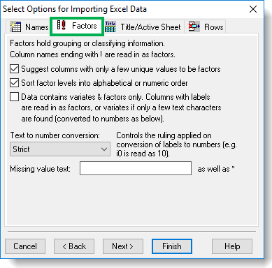
| Suggest columns with only a few unique values to be factors |
Genstat will prompt you to convert columns to factors when the column contains x number of repeated values. You can set the number of repeated values in Tools | Spreadsheet Options then click the Conversions tab. Select Suggest converting columns with <=x unique items to factors and set the number as required. |
| Sort factor levels into alphabetical or numeric order |
If your data contains factor columns this option will sort the numeric levels (or text labels) into ascending order. |
| Data contains variates & factors only | Any column containing text will be converted to either a variate or factor. If the column contains less than 20% text cells, the column will be made into a variate, otherwise the column will be made into a factor |
| Text to number conversions | Sometimes numbers are accidentally mistyped as letters. Common mistypings include i, I, l, L for the number 1; o, O for the number 0; a comma for a decimal point, etc. Text to number allows Genstat to convert text labels by substituting numbers for letters or, where this is not possible, the label is converted to a missing value. Strict – Change text strings to numbers only when there are no non-numeric characters in the string. For example, the text ’23’ is converted to 23, the text ‘1a’ contains an alphabetic character so the whole label is converted to a missing value. 1 substitution – Allow a single number to be mistyped and substitute this with the appropriate number. A single lower case ‘o’ or upper case ‘O’ is converted to 0: lower case ‘i’, upper case ‘I’, lower case ‘l’, or upper case ‘L’ is converted to 1. Lower case ‘s’ or upper case ‘S’ is converted to 2. A comma is converted to a decimal point. For example, ‘1o’ contains a single alphabetic character so is converted to 10, ‘1,i’ contains two a comma and an alphabetic characters so is converted to a missing value. Common substitutions – Allows multiple numbers to be mistyped and converts them to the appropriate numbers. For example, ‘LOO’ is converted to 100. Standard – The same as Common substitutions, but any letters at the end of a number are ignored. For example, ’23o’ is converted to 23, ‘i20’ has an alphabetic character at the front so the whole label is converted to a missing value. Lax – Change all text numbers to actual numbers and remove any non-numeric characters. For example, ‘A23X’ is converted to 23. |
| Missing value text | This lets you supply your own text to be inserted into empty cells (the default values are an asterisk * for a variate column or a blank cell for factors and texts). For example, you could use N/A to represent a missing value. |
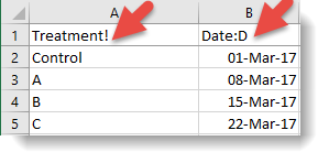
Additional information about column data type conversions
Columns whose names are suffixed with a ! character will be automatically converted into factors. Similarly, if column names end with a $ or # character, then these will be converted into a text and variate respectively. As well as supplying a conversion character, column format information can be appended to a column name. For example, a suffix of :0, :1, :2 … :9 specifies that the column should be displayed with the given fixed number of decimal places. These column markers are summarized in the table below.
| ! | Interpret the column as a factor |
| # | Interpret the column as a variate |
| $ | Interpret the column as a text |
| :D | Display the column as a date |
| :T | Display the column as a time |
| :0, :1, :2…:9 | Display the column with a fixed number of decimal places |
| :E | Display the column in scientific format |
The ! marker can be applied in conjunction with the Date :D or Time :T markers, so that !:D would indicate a factor with levels displayed as dates.
In the Excel spreadsheet below, column A will be imported into Genstat as a factor while column B will be imported as a date.
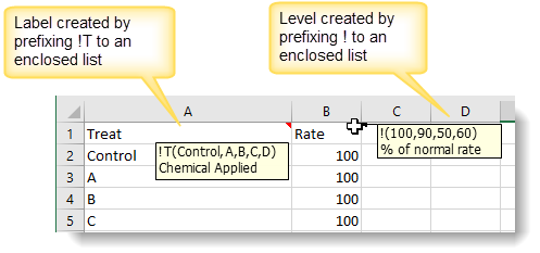
You can specify the order of factor levels and labels within an Excel file by adding a comment to the cell that contains the column name. Within the comment the factor levels must start with a ! and labels must start with !t on a new line. The levels and labels should then be entered within brackets. For example, for levels this could be !(100,90,50,10) and for labels this could be !T(Control,A,B,C) or !t(‘Control’,’A’,’B’,’C’). The order of the items in the comment will define the order of the levels or labels in the factor. If a column only contains ordinal values (i.e. 1…n), then the comment can still be used to assign labels or levels to these groups. The first item in the comment will define the level or label for group 1 in the factor and so on.
A column description can also be supplied in the comment as a separate line, but this must not start with an exclamation mark.
The following image shows two comments entered into Excel (to do this right-click and select Insert Comment, making sure you don’t put line breaks in the middle of the list). Each column will be opened in Genstat as a factor using the defined levels/labels and will include a column description. Refer to Using Excel Cell Comments with Genstat for more information about setting up comments.
This controls some general features available for the spreadsheet.
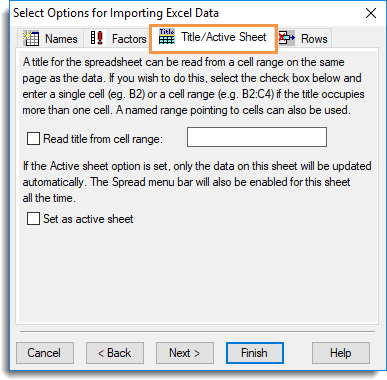
| Read title from cell range | The cell range you specify (e.g. A2:B3) or named range (which must be located on the same sheet as the data) will be used to read text for the spreadsheet title. Note that text for the different cells within this range will be concatenated. |
| Set as active sheet | This sets the new spreadsheet that is created as the active spreadsheet. Setting an active spreadsheet provides a method of avoiding multiple data updates to the server when more than one spreadsheet is open within Genstat. When a spreadsheet is set as the active spreadsheet only data from that spreadsheet is automatically updated to the Genstat server. Another advantage of specifying an active spreadsheet is that the Spread menu options and spread toolbar buttons will always be enabled even if your spreadsheet does not have the cursor focus |
These options control which rows of data are read into the new spreadsheet.
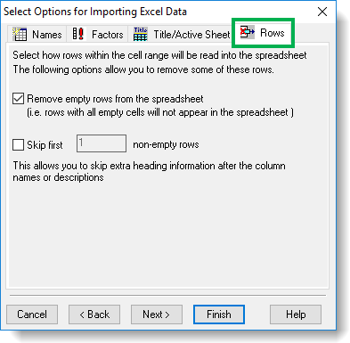
| Remove empty rows from the spreadsheet | Remove any rows that contain no data. Deselect this option if you want to import the empty rows. |
| Skip first X non-empty rows | The first specified number of rows will be excluded from the spreadsheet. This is useful to exclude any comments that made have been made in the worksheets. Text in these rows can still be used for column names or descriptions. |