Non-hierarchical Cluster Analysis

Select menu: Stats | Multivariate Analysis | Cluster Analysis | Non-hierarchical

Non-hierarchical cluster analysis forms a grouping of a set of units, into a pre-determined number of groups, using an iterative algorithm that optimizes a chosen criterion. Starting from an initial classification, units are transferred from one group to another or swapped with units from other groups, until no further improvement can be made to the criterion value.

The method is explained in more detail in The Guide to Genstat, Part 2: Statistics, which you can open as a PDF file from the menu Help | Genstat Guides | Statistics. There is no guarantee that the solution thus obtained will be globally optimal – by starting from a different initial classification it is sometimes possible to obtain a better classification. However, starting from a good initial classification (see Options) much increases the chances of producing an optimal or near-optimal solution.

After you have imported your data, from the menu select
Stats | Multivariate Analysis | Cluster Analysis | Non-hierarchical.
OR
Stats | Data Mining | Cluster Analysis | Non-Hierarchical.
Fill in the fields as required then click Run.

You can set additional Options before running the analysis and store the results by clicking Store.

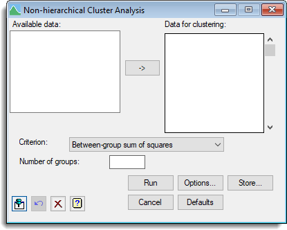
Data for clustering

Specifies the set of variates making up the data matrix. The names of the variates can be selected from Available data. You can transfer multiple selections from Available data by holding the Ctrl key on your keyboard while selecting items, then click to move them all across in one action.

Criterion

The criterion to be optimized by the clustering. This can be set to one of the following four choices:

Within-class dispersion	Minimizes the determinant of the pooled within-class dispersion matrix (W). Under the assumption that the data originated from a mixture of k multivariate Normal distributions, with equal variance-covariance matrix V, the MLE of V is obtained when the grouping into k classes minimizes det(W). Obtains compact groups.
Mahalanobis squared distance	Maximizes the total between-groups Mahalanobis squared distance. This will obtain separation of groups, possibly at the cost of compactness. Equivalent to the Within-class dispersion criterion when there are only two groups.
Between-group sum of squares	Minimizes the trace of the pooled within-class dispersion matrix (W). Equivalent to maximizing the total between-group sum of squares, or Euclidean distance between groups.
Maximal predictive classification	Maximal predictive classification is suitable for binary data. Each group has a class predictor, a binary indicator for each variate set to 0 or 1 according to whichever value is more frequent in the group. The criterion to be maximized is the total number of agreements between units and their respective class predictors.

Number of groups

Sets the number of groups to be formed.

Action buttons

Run	Run the analysis.
Cancel	Close the dialog without further changes.
Options	Opens the Options dialog where you can control various aspects of the algorithm used for the clustering, specify the initial classification and also select which results are to be printed.
Defaults	Reset options to the default settings. Clicking the right mouse on this button produces a shortcut menu where you can choose to set the options using the currently stored defaults or the Genstat default settings.
Store	Opens a dialog where you can store results from the analysis.

Action Icons

	Pin	Controls whether to keep the dialog open when you click Run. When the pin is down the dialog will remain open, otherwise when the pin is up the dialog will close.
	Restore	Restore names into edit fields and default settings.
	Clear	Clear all fields and list boxes.
	Help	Open the Help topic for this dialog.