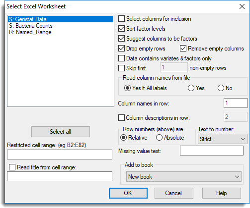
Prior to the introduction of the Excel import wizard, the Select Excel Worksheet dialog was the standard way of importing Excel or Quattro Windows files. This legacy dialog is still available for users who are more comfortable using this import method.
- To turn off the Excel import wizard and use the legacy dialog, select Tools | Spreadsheet Options, click the Sheets tab then deselect Use Import Wizard when opening an Excel file.
The Select Excel Worksheet dialog will then display in place of the Excel import wizard whenever you open an Excel or Quattro Windows file (WQ1, WB1/2/3). An explanation of each option on this dialog is given further down the page.
Both of these file formats can contain several worksheets. Worksheets and named ranges are shown in the preview pane prefixed by S: and R: respectively (see image below).
If a single worksheet or named range is to be opened you can specify a sub-range of the data to be loaded.
If you have any named ranges in the file then these have the advantage that both the sheet and cell range are specified permanently in the Excel file. These are automatically updated if further rows or columns are inserted into the cell range.
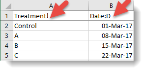
Columns whose names are suffixed with a ! character will be automatically converted into factors. Similarly, if column names end with a $ or # character, then these will be converted into a text and variate respectively. As well as supplying a conversion character, column format information can be appended to a column name. For example, a suffix of :0, :1, :2 … :9 specifies that the column should be displayed with the given fixed number of decimal places. These column markers are summarized in the table below.
| ! | Interpret the column as a factor |
| # | Interpret the column as a variate |
| $ | Interpret the column as a text |
| :D | Display the column as a date |
| :T | Display the column as a time |
| :0, :1, :2…:9 | Display the column with a fixed number of decimal places |
| :E | Display the column in scientific format |
The ! marker can be applied in conjunction with the Date :D or Time :T markers, so that !:D would indicate a factor with levels displayed as dates. In the Excel spreadsheet below, column A will be imported into Genstat as a factor while column B will be imported as a date.
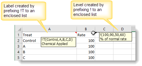
You can specify the order of factor levels and labels within an Excel file by adding a comment to the cell containing the column name. Within the comment the factor levels must start with a ! and labels must start with !t on a new line. The levels and labels should then be entered within brackets.
For example, for levels this could be !(100,90,50,10) and for labels this could be !T(Control,A,B,C) or !t(‘Control’,’A’,’B’,’C’). The order of the items in the comment will define the order of the levels or labels in the factor. If a column just contains ordinal values (i.e. 1…n), then the comment can still be used to assign labels or levels to these groups. The first item in the comment will define the level or label for group 1 in the factor and so on.
A column description can also be supplied in the comment as a separate line, but this must not start with an exclamation mark.
The following image shows two comments entered into Excel (to do this right-click and select Insert Comment, making sure you don’t put line breaks in the middle of the list). Each column will be opened in Genstat as a factor using the defined levels/labels and will include a column description. Refer to Using Excel Cell Comments with Genstat for more information about setting up comments.
| Select all | Select all items within the list of worksheets and named ranges. |
| Restricted cell range | You can load a subset of the data from a worksheet by specifying the position of diagonally opposite corners of the rectangle that spans the required range. For example B12:E18 will load seven rows and five columns starting at row 12 of the second column. You can also enter partial column or row information:
|
| Read title from cell range | The cell range you specify (e.g. A2:B3) or named range (which must be located on the same sheet as the data) will be used to read text for the spreadsheet title. Note that text for the different cells within this range will be concatenated. |
| Select columns for inclusion |
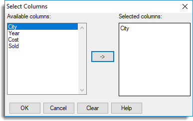
Lets you select a subset of columns from the worksheet. When you click OK the Select Columns dialog will open to allow you to select the required columns.
|
| Sort factor levels | If your data contains factor columns this option will sort the numeric levels (or text labels) into ascending order. |
| Suggest columns to be factors | Genstat will prompt you to convert columns to factors when the column contains x number of repeated values. You can set the number of repeated values in Tools | Spreadsheet Options then click the Conversions tab. Select Suggest converting columns with <=x unique items to factors and set the number as required. |
| Drop empty rows | Remove any rows that contain no data. |
| Remove empty columns | By default, any columns that do not contain data are removed from the Genstat spreadsheet. However, you can keep the empty columns by deselecting this option. |
| Data contains variates & factors only | Any column containing text will be converted to either a variate or factor. If the column contains less than 20% text cells, the column will be made into a variate, otherwise the column will be made into a factor. |
| Skip first x non-empty rows | The first specified number of rows will be excluded from the spreadsheet. This is useful to exclude any comments that made have been made in the worksheets. Text in these rows can still be used for column names or descriptions – see next option below. |
| Read columns names from file | Controls whether the imported column names are used. Yes if all labels – Read the column names from the row specified in the Column names in row option if all the cells in this row contain labels only or are empty. A default column name will be generated for an empty cell. Yes – Use the cells specified in the Column names in row option . If a cell contains a number, then it will be prefixed with “_” to ensure it is a valid Genstat identifier name. No – Generate default names for the columns, ignoring those in the file. |
| Column names in row | Specifies the row number to use for column names. |
| Column descriptions in row | When selected, the cells in the specified row number will be used for column descriptions. |
| Row numbers (above) are | Controls whether the row numbers are relative to the data range or relate to a whole worksheet. Relative – Row numbers start from the top of the restricted cell range. Absolute – Row numbers start from the top of the worksheet and thus correspond to the absolute row numbering in Excel/Quattro. |
| Text to number | Sometimes numbers are accidentally mistyped as letters. Common mistypings include i, I, l, L for the number 1; o, O for the number 0; a comma for a decimal point, etc. Text to number allows Genstat to convert text labels by substituting numbers for letters or, where this is not possible, the label is converted to a missing value. Strict – Change text strings to numbers only when there are no non-numeric characters in the string. For example, the text ’23’ is converted to 23, the text ‘1a’ contains an alphabetic character so the whole label is converted to a missing value. 1 substitution – Allow a single number to be mistyped and substitute this with the appropriate number. A single lower case ‘o’ or upper case ‘O’ is converted to 0: lower case ‘i’, upper case ‘I’, lower case ‘l’, or upper case ‘L’ is converted to 1. Lower case ‘s’ or upper case ‘S’ is converted to 2. A comma is converted to a decimal point. For example, ‘1o’ contains a single alphabetic character so is converted to 10, ‘1,i’ contains two a comma and an alphabetic characters so is converted to a missing value. Common substitutions – Allows multiple numbers to be mistyped and converts them to the appropriate numbers. For example, ‘LOO’ is converted to 100. Standard – The same as Common substitutions, but any letters at the end of a number are ignored. For example, ’23o’ is converted to 23, ‘i20’ has an alphabetic character at the front so the whole label is converted to a missing value. Lax – Change all text numbers to actual numbers and remove any non-numeric characters. For example, ‘A23X’ is converted to 23. |
| Missing value text | This lets you supply your own text to be inserted into empty cells (the default values are an asterisk * for a variate column or a blank cell for factors and texts). For example, you could use N/A to represent a missing value. |
| Add to book | Any open spreadsheets will be displayed in this dropdown list. Select a spreadsheet to insert your data into or leave it at the default setting New Book to create a new workbook. |