Linear Regression with Correlated Errors

Select menu: Stats | Repeated Measurements | Linear Regression with Correlated Errors

Use this to fit regression models to data, such as repeated measurements, where the residuals may follow an AR1 or a power-distance correlation model.

After you have imported your data, from the menu select
Stats | Repeated Measurements | Linear Regression with Correlated Errors.
Fill in the fields as required then click Run.

You can set additional Options then after running, you can save the results by clicking Save.

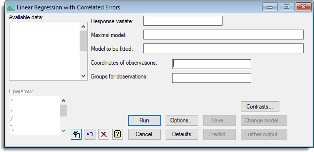
The coordinates of the observations in the direction (e.g. time) along which the correlation model operates should be supplied. Also a factor can be specified to define groups of observations for the model – the correlation model is then defined only over the observations that belong to the same groups. You can specify your own models in command mode using the RAR1 procedure.

Available data

This lists data structures appropriate to the current input field. It lists either variates for specifying the response or explanatory variate, or a factor for specifying groups. The contents will change as you move from one field to the next. Double-click a name to copy it to the current input field or type the name.

Response variate

Specifies the name of the response (or y-) variate.

Maximal model

The maximal model lets you specify the most complicated model that you are likely to want to consider. When a maximal model is supplied the terms displayed within the Change model dialog will only be those specified within the maximal model.

Model to be fitted

Specifies the model to be fitted by entering a model formula. The formula can involve both variates and factors which can be selected from the Available data list, and operators from the Operators list. A variate in the formula represents its linear effect, and a factor represents its main effect: that is, a separate intercept for each level of the factor. An interaction between factors allows separate intercepts for each combination of levels of the factors. An interaction between a variate and a factor represents separate slopes for each level. You can also include interactions between variates, representing the linear effect of the product of the two variates, and interactions between any number up to nine variates and factors.

Coordinates of observations

A variate specifying the coordinates of the observations in the direction (e.g. time) along which the correlation model operates.

Groups for observations

A factor to define groups of observations for the model – the correlation model is then defined only over the observations that belong to the same groups.

Operator list

This list operators that can be used to construct a model formula for the model to be fitted and maximal model. There are also functions available that provide more general effects of variates than a linear effect. The POL() function represents polynomial effects up to the order given in the second argument (maximum 4); so POL(x; 3) represents a cubic effect of the variate x. The REG() function represents orthogonal polynomials (maximum order 8). The COMP() function can be used to estimate comparisons.

The S() function represents nonparametric effects, fitted by cubic smoothing splines, with the number of degrees of freedom specified; so S(x; 4) represents a smoothed effect of x with 4 d.f. (also called an additive effect of x). The POL and REG functions cannot be combined in interaction terms, but the S function may appear in interactions with factors, when the linear effect of the variate is estimated separately for each level together with a single smoothed effect for all levels.

Contrasts

Lets you construct contrasts. This generates a menu that lets you choose between different types of contrasts to use in the analysis.

Action buttons

Run	Run the analysis.
Cancel	Close the dialog without further changes.
Options	Opens a dialog where additional options and settings can be specified for the analysis.
Defaults	Reset options to the default settings. Clicking the right mouse on this button produces a shortcut menu where you can choose to set the options using the currently stored defaults or the Genstat default settings.
Save	Opens a dialog where you can save results from the analysis.
Predict	Allows you form predictions based on the current regression model.
Change model	After fitting the model you can investigate other models by using the Change Model dialog to add or drop terms from the model. Note that the parameter phi is estimated for the initial model that is fitted and is fixed for models that are altered using the Change model dialog.
Further output	Opens a dialog for specifying further output from the analysis and displaying residual and fitted model graphs.

Action Icons

	Pin	Controls whether to keep the dialog open when you click Run. When the pin is down the dialog will remain open, otherwise when the pin is up the dialog will close.
	Restore	Restore names into edit fields and default settings.
	Clear	Clear all fields and list boxes.
	Help	Open the Help topic for this dialog.