Select menu: Spread | Column | Conditional Formatting
This menu allows numbers within a spreadsheet column to be coloured according to a set of conditional rules.
- From the menu select Spread | Column | Conditional Formatting.
Up to three rules can be applied to a column, although the between rule counts as two. The rules are applied sequentially, so that if the first rule applies, that is the colour used. Thus the ordering of rules can be important. For example the rules “Greater than 10“, “Greater than 20” and “Greater than 30” in that order would not give the required three colours, as all values greater than 20 or 30 meet the first condition and so would be just coloured in the first specified colour. To get three colours the rules would need to be in the order of the most restrictive to the least, i.e. “Greater than 30“, “Greater than 20” and “Greater than 10“. The conditional formatting details are saved in a Genstat spreadsheet (GSH) or book (GWB) file and will be displayed when the spreadsheet is reopened.
The background shading options allow you to set coloured backgrounds for the cells in each column, based on the where the cell values falls between the specified shading minimum and maximum values. The colour saturation value controls the intensity of colour used, 100% being maximum intensity, and lower values giving lighter pastel colours.
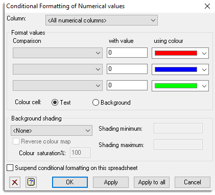
Column
This lists columns in the current spreadsheet. Select the column that is to be conditionally formatted from the list. If the spreadsheet contains selected columns then select the All selected columns item to apply the conditional formatting to all the selected columns. Also, the option All numerical columns can be selected to apply the conditional formatting to all the numerical columns within a spreadsheet.
Format values
Specifies the rules to be used for the colouring of the cells.
| Comparison | A list of possible comparisons to use for the conditional formatting. If the blank item is selected then no comparison is performed. A list of available comparisons is given below. |
| with value | The value that the column items are compared with. If the comparison is true, then the column value will be displayed in the specified colour. |
| using colour | Lists the colours that can be used when the conditional statement is true. |
| Colour cell | This controls whether the conditional formatting is applied to cell text or the cell background. |
The available comparisons for the formatting include:
| Equals (==) | The column value is equal to the specified value. |
| Less than (<) | The column value is less than the specified value. |
| Greater than (>) | The column value is greater than the specified value. |
| Less than or equals (<=) | The column value is less than or equal to the specified value. |
| Greater than or equals (>=) | The column value is greater than or equal to the specified value. |
| Between and | This item requires two specified values and is true when the column value falls between these two values. |
Background shading
These options allow you to specify a colour scheme to use to colour the cell backgrounds for a column. If the Colour cell is set to background then the background shading will not be used for those cells
The dropdown list provides a range of colour series interpolated between the shading minimum and maximum values. The maps available are:
| Blue-Red Map | Blue to white to red. |
| Heat Map | Blue to green to red to yellow to white. |
| Topographical Map | Blue to green to brown. |
| Rainbow Map | Red to orange to yellow to green to blue to indigo to violet. |
| Outlier Map | Values equal to or below the shading minimum are coloured blue, and those equal to or above the maximum are shaded red. |
Other background shading options include:
| Shading minimum | The minimum value used in the colour shading. Values close to, or below the minimum value will be given the first colour in the colour map. |
| Shading maximum | The maximum value used in the colour shading. Values close to, or above the maximum value will be given the last colour in the colour map. |
| Reverse colour map | When selected, the colour list will be reversed. For example, the Blue-Red map will go from red for the minimum to blue for the maximum. |
| Colour saturation (%) | The colour saturation value controls the intensity of colour used. A value of 100% gives the maximum intensity with bright colours, and lower percentages giving lighter pastel colours. |
Suspend conditional formatting on this spreadsheet
When selected, the conditional formatting is suspended on all columns. This provides an easy method of turning off the formatting temporarily, whilst retaining the ability to re-enable it at a later date.
Action buttons
| OK | Apply the specified conditional formatting on the selected column and close the dialog. |
| Apply | Apply the specified conditional formatting on the selected column. |
| Apply to all | Apply the specified conditional formatting to all the columns in the spreadsheet and close the dialog. |
| Cancel | Close the dialog without further changes. |
See also
Bookmark Spreadsheet by Value
Options – Fonts and Colours
Spreadsheet Column Menu
Cell Colours
Column Colours
Factor Background Colours