Select menu: Stats | Time Series | Moving Average
Use this to calculate a moving average of a time series.
- After you have imported your data, from the menu select
Stats | Time Series | Moving Average. - Fill in the fields as required then click Run.
You can set additional Options before running and store the results by clicking Store.
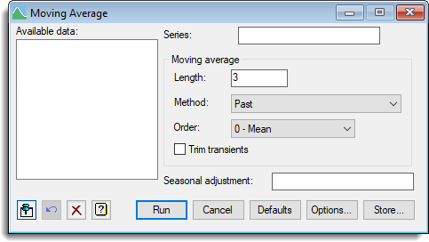
Available data
This lists variates that can be used for the data and save input fields. Double-click a name to copy it into the current input field or type the name.
Series
Specifies a variate containing a time series for which the moving average is to be calculated.
Length
Number of samples in the moving average. For a centred moving average, with order > 0, this must be an odd number. The number of samples must be greater than the order of the moving average.
Method
This specifies the type of moving average to be calculated. The options are:
| Past | An unweighted average of the past values, |
| Centred | An average centred on the current value with the first and last samples receiving weights of 0.5 when the length is even, |
| Exponential | An exponentially weighted average of past values, |
| Filter | Uses FILTER to smooth the data using a specially constructed ARIMA model. |
| Holt-Winters (double exponential) | A Holt-Winters filter to smooth the data. This model fits separate level, trend, and seasonal components, each exponentially weighted with parameters alpha, beta and gamma respectively. See the MOVINGAVERAGE procedure for a fuller description of this filter. |
Order
The order for polynomial smoothing. Setting the order to 0 will produce an ordinary moving average calculated from means.
Trim transients
For the past or centred methods with order 0, this option trims transients and the start (or end for centred) of the series. Transients are those points that are not fully estimated as they do not have the full set of samples before or around them.
Seasonal adjustment
This specifies a factor that will be used to adjust the moving average. The residuals (the observed values minus the moving average) are calculated and then averaged for each level of this factor. These averages for each level are then removed from the corresponding units of the moving average so that the mean residual for each level will now be zero.
Action buttons
| Run | Calculate the moving average. |
| Cancel | Close the dialog without further changes. |
| Defaults | Change the options in the menu to their defaults. Right clicking on this button allows the selection of either User or Genstat defaults. |
| Options | Open the Options dialog. |
| Store | Open the Store dialog to save output from the analysis. |
Action Icons
| Pin | Controls whether to keep the dialog open when you click Run. When the pin is down |
|
| Restore | Restore names into edit fields and default settings. | |
| Clear | Clear all fields and list boxes. | |
| Help | Open the Help topic for this dialog. |
Example
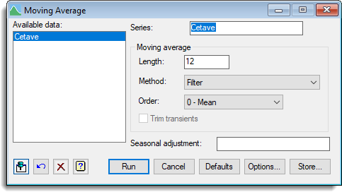
The file ‘Cetave.dat’ gives the monthly mean temperature of Central England for 1659-1973.
- From the menu select Data | Load | ASCII File.
- Click Browse and navigate to the default installation folder, which will be (on a Windows PC)
C:\Program Files\Gen20Ed\Examples\GuidePart2\cetave.dat. - Enter ‘Cetave’ as the Names for data columns then click Open.
- Now select Stats | Time Series | Moving Average. and fill out the dialog as shown below.
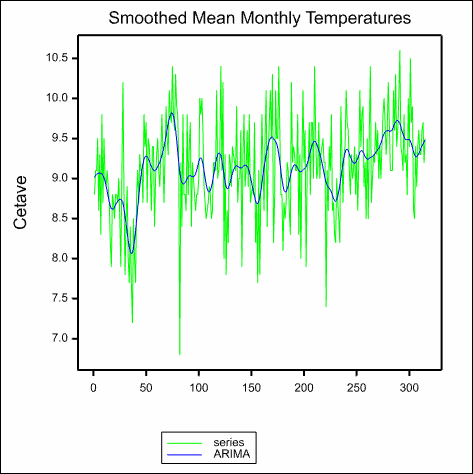
- Click Options and enter the Graph title as ‘Smoothed Mean Monthly Temperatures‘ then click OK and Run to produce the graph.
The moving average of length 12 is chosen to average over a year’s data to make it less sensitive to the monthly variation over the year.
See also
- Moving Average Options dialog.
- Moving Average Store Options dialog.
- Data Exploration of a time series menu.
- ARIMA menu.
- MOVINGAVERAGE procedure