Nonlinear Quantile Regression

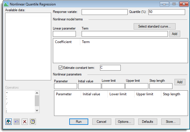
Select menu: Stats | Regression Analysis | Nonlinear Quantile Regression

This dialog allows a nonlinear quantile regression model to be fitted.

After you have imported your data, from the menu select
Stats | Regression Analysis | Nonlinear Quantile Regression.
Fill in the fields as required then click Run.

You can set additional Options before running the analysis and store the results by clicking Store.

To help with the selection of an appropriate nonlinear curve you can examine example plots to see a range of nonlinear models, otherwise you can enter your own calculation for the nonlinear terms.

This menu fits models of the form Y = A*F(X;P;Q;…) + B*G(W;R;S…) + … + C. The terms which are nonlinear functions of data variates and unknown parameters are given via a series of calculations. The scalars that are the nonlinear parameters (P,Q,R,S in the above example) are entered into the nonlinear parameter list along with initial values or bounds. The scalars which hold the linear parameters (the coefficients A and B in the above formula) are specified for each term, and for the constant, if fitted.

The terms need not all have nonlinear parameters, as a mix of linear and nonlinear terms can be specified. For example a exponential plus line can be fitted by specifying two terms, EXP(C*X) and X. The menu assumes that each calculation expression in each term is a separate predictor of Y, and so if you need to create intermediate calculation terms to generate the predictors, then you will need to use the RQNONLINEAR procedure in an input window, as this allows more flexibility in the specification of the model.

The options control the output and which graphs are printed and whether bootstrapping is used to calculate standard errors, confidence limits and correlations. A choice of optimization algorithm is also available in the options.

If the model does not converge then different initial values or reducing the step length can help, or else changing the optimization algorithm. The simplex model can be slower to converge but in some cases converges more surely that the GaussNewton algorithm. The simplex algorithm only requires bounds for each nonlinear parameter, but the other algorithms require an initial value. If using a standard model, then you can fit the parameters for the mean model using the Standard Curves menu, or for general nonlinear models use the Nonlinear models menu to estimate the parameters for the mean model and use these as initial values for the quantile model.

Available data

This lists data structures appropriate to the current input field. It lists either variates for specifying the response variate, items in the terms calculation, or scalars for the parameters. The contents will change as you move from one field to the next. Double-click a name to copy it to the current input field or type the name.

Response variate

Specifies the name of the variate containing the response (y) values.

Quantile (%)

Percentage between 0 and 100 at which to calculate quantiles; default 50%.

Select standard curve

Opens a dialog for specifying a standard curve to be fitted. This fills in the terms and parameters using the parameterization as specified in the FITCURVE directive. For robustness of fitting some transforms of the parameters are fitted for some models. For example rather than fitting Y = A + B*R**X as in the Standard curve menu, the formulation Y = A + B*EXP*(C*X) is used with C = log(R). The initial values for the parameters could be obtained by fitting the model using the Standard Curves menu. There are five general classes of curve; each has several variations.

Nonlinear model terms

List of the expressions that are fitted additively to the Response variate, and their linear parameter (the coefficient that multiplies the term in the model). The terms contain the calculations involving the nonlinear parameters. To create a term give a name for a scalar to hold the linear parameter and the calculation for the term then click the Add button.

To edit a term click on its row in the list, and the item will be placed in the Linear parameter and Term fields. Modify the entries, and click the Add button to re-enter the item. If the linear parameter name has changed this will create a new entry, otherwise the old entry will be modified. To remove an entry, select the row (or rows for multiple deletions) and either right click the list and select the Delete selection or Delete all menu items, or press your keyboard Backspace key.

Linear parameter

A scalar that will hold the linear parameter for each term. The linear parameter is the coefficient that multiplies the term in the model. This is estimated by the model fitting process.

Term

The calculation that gives the predictors to be additively fitted to the response variate. This can be any formula that the CALCULATE directive can evaluate. It need not involve the nonlinear parameters, it can just be a single variate like X if a linear term is required. It must produce a variate of the same length as the response variate. It may involve other scalars which have fixed values, and are not to be estimated.

For example, for an exponential model Y = A + B*EXP(C*X), the term would be EXP(C*X), with linear parameter B and constant A. There would be one nonlinear parameter C.

For example, for an exponential model with Y = A + B*EXP(C*X) + D*X, there would be two term EXP(C*X) and X, with linear parameter B and D respectively and constant A.

For example, for an critical exponential model with Y = A + B*(1 + D*X)*EXP(C*X), there would be one term (1 + D*X)*EXP(C*X), with linear parameter B and constant A. There would be two nonlinear parameters C and D.

Estimate constant term

Whether to estimate a constant as part of the regression model. The edit field contains the name of a scalar which will hold the fitted constant.

Nonlinear parameters

This section, you specify the name, initial values, upper & lower bounds and step length for each nonlinear parameter used in the term calculations, and then add it to the list using the Add button. To create a nonlinear parameter give a name for a scalar to hold the linear parameter, and the initial value (not required for the simplex algorithm) and the bounds (required for the simplex algorithm, but otherwise optional), and optionally the step length, and then use the Add button. To edit a parameter click on its row in the list, and the items will be place in the Parameter – Step length fields. Modify the entries, and click the Add button to reenter the parameter. If the parameter name has changed this will create a new entry, otherwise the old entry will be modified. To remove an entry, select the row (or rows for multiple deletions) and either right click the list and select the Delete selection or Delete all menu items, or press your keyboard Backspace key.

Parameter

Enter the name of a scalar for the nonlinear parameter that is to be estimated. The parameter name must occur in one of the terms.

Initial value

The initial value of the parameter. This must be set unless the simplex algorithm is being used. This is not used for the simplex algorithm.

Lower & upper limits

Provides fixed limits for the search. These must be set when the simplex algorithm being used, and are used to initialize the points on the simplex, but otherwise is optional.

Step length

Optional initial step lengths for the search. If these are set to missing (showing as *) then by default the step length is 0.05 times the initial value of the parameter, or 1.0 if the initial value is zero. This is not used for the simplex algorithm.

Operators

This provides a quick way of entering operators in the term calculation. Double-click on the required symbol to copy it to the term input field. You can also type in operators directly.

Action buttons

Run	Run the analysis.
Cancel	Close the dialog without further changes.
Options	Opens a dialog where additional options and settings can be specified for the analysis.
Defaults	Reset options to the default settings. Clicking the right mouse on this button produces a shortcut menu where you can choose to set the options using the currently stored defaults or the Genstat default settings.
Save	Opens a dialog where you can store results from the analysis.

Action Icons

	Pin	Controls whether to keep the dialog open when you click Run. When the pin is down the dialog will remain open, otherwise when the pin is up the dialog will close.
	Restore	Restore names into edit fields and default settings.
	Clear	Clear all fields and list boxes.
	Help	Open the Help topic for this dialog.

Examples

The Genstat spreadsheet file ‘Nonlinear Models.gsh‘ in the Genstat Examples directory contains a number of Y variates that depend on the variate X and follow various nonlinear models.

From the menu select File | Open then navigate to the default Windows installation folder C:\Program Files\Gen20Ed\Examples and select Nonlinear Models.gsh.
From the menu select Stats | Regression Analysis | Nonlinear Quantile Regression.
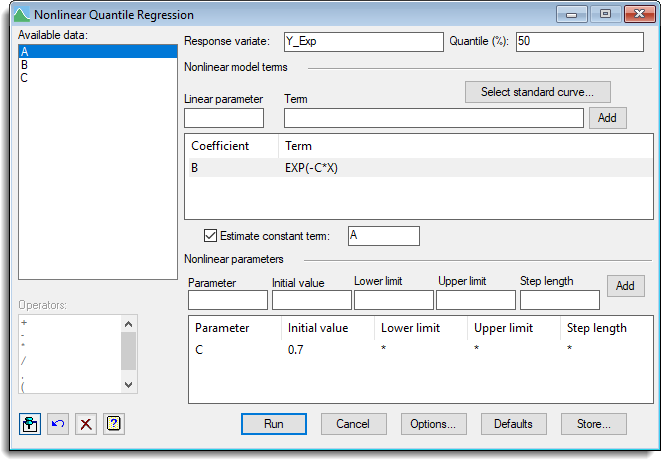
To fit an exponential model Y = A + B*EXP(-C*X) to the response variate Y_Exp, set options as follows:
Enter Y_Exp into the Response variate field.
Enter the nonlinear predictor EXP(-C*X) into the Term field, its multiplier B into the Linear parameter field then click the Add button beside the Term field.
Tick the box Estimate constant term and enter the constant name A.
Enter the nonlinear parameter C into the Parameter field, give it an Initial value of 0.7 then click the Add button in this section.
The Lower bound, Upper bound and Step length fields can be left empty as they are not required for the Gauss-Newton algorithm and any value of C is valid in the function.
Click Options, tick the box for Bootstrap confidence intervals and enter 500 as the Maximum number of iterations.
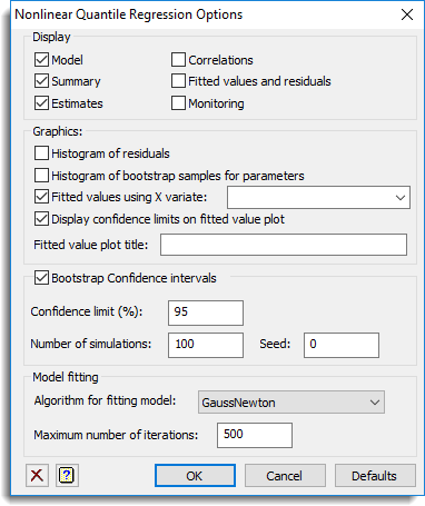
Click OK to close this dialog then click Run.

Running this analysis produces the resulting graph.

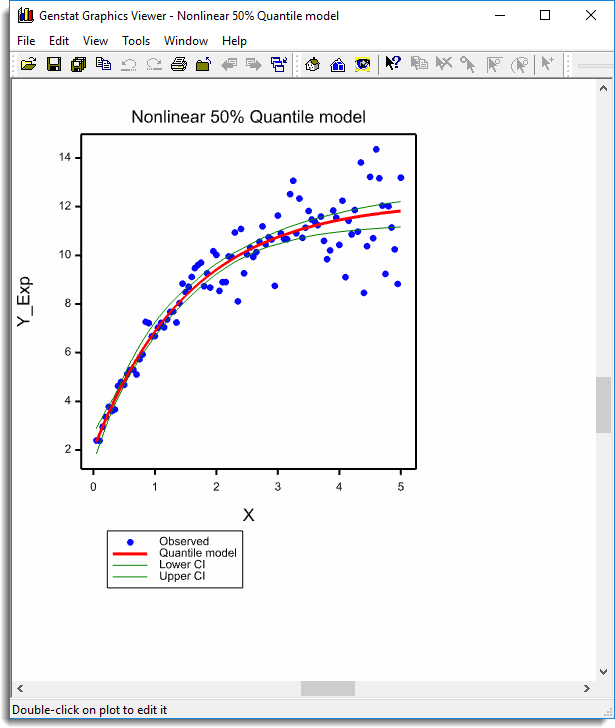
The parameter estimates and confidence limits can be found in the Output window.

Note: Running this analysis may produce an error message such as:

“Warning 3, code UF 2, statement 227 in procedure RQNONLINEAR The model failed to fit to 6 bootstrap samples”

This is normal. As a random sample is generated in the bootstrap process, the model will not fit on some of these. Unless you specify a seed to generate the same set of samples each time, the number of failures will vary from run to run. This is expected with a nonlinear model, which is quite complicated to fit, and some fits get lost look for the optimal spot on the non-linear surface.