Select menu: Stats | Regression Analysis | Standard Curves
This menu allows a variety of standard nonlinear regression models to be fitted. You can specify your own models using command mode, either with the FIT or FITNONLINEAR directives.
- After you have imported your data, from the menu select
Stats | Regression Analysis | Standard Curves. - Fill in the fields as required then click Run.
You can set additional Options then after running, you can save the results by clicking Save.
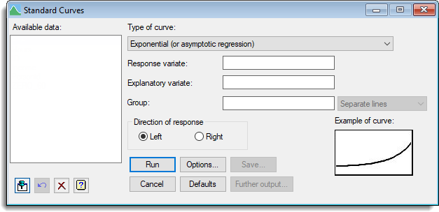
Available data
This lists data structures appropriate to the current input field. It lists either variates for specifying the response or explanatory variate, or a factor for specifying groups. The contents will change as you move from one field to the next. Double-click a name to copy it to the current input field or type the name.
Type of curve
This is used to select the type of curve to be fitted. There are five general classes of curve; each has several variations.
To help with the selection of an appropriate curve you can examine example plots of each type.
Response variate
Specifies the name of the variate containing the response (y) values.
Explanatory variate
Specifies the name of the variate containing the explanatory (x) values.
Group
For data classified into groups, different curves can be fitted to each group, possibly constrained by restricting some of the parameters to values common to all groups. The groups are specified using a factor.
The first model to be fitted is a single curve with common parameters over all the groups. Next the model is extended to include a different constant parameter for each group, giving a set of parallel curves, one for each group. The next model has all linear parameters, including the constant, different for each group. (The linear parameters are those, like b in the exponential curve, with respect to which the model is linear.) Finally, completely separate curves are fitted, in which all the parameters differ between groups. The list adjacent to the Group field lets you select between the types of regression model that you want to fit.
Graphs and further output from this analysis will display information from the final (full) model. The accumulated display setting is particularly useful, producing an accumulated analysis of variance which lets you assess how complicated a model is really needed. The final line of the table checks whether separate nonlinear parameters are needed. If these are not required, the previous line, representing the interaction between the explanatory variate and the groups factor, can be used to assess whether separate linear parameters are required. If not, the line before that, representing the main effect of the groups factor, assesses whether different constants are needed. You can use FITCURVE in command mode to fit a particular sub-model, for example:
FITCURVE [CURVE=logistic] variate + factor
fits separate constants for each group, giving the parallel curves model.
Action buttons
| Run | Run the analysis. |
| Cancel | Close the dialog without further changes. |
| Options | Opens a dialog where additional options and settings can be specified for the analysis. |
| Defaults | Reset options to the default settings. Clicking the right mouse on this button produces a shortcut menu where you can choose to set the options using the currently stored defaults or the Genstat default settings. |
| Save | Opens a dialog where you can save results from the analysis. |
| Further output | Opens a dialog for specifying further output from the analysis and displaying residual and fitted model graphs. |
Action Icons
| Pin | Controls whether to keep the dialog open when you click Run. When the pin is down |
|
| Restore | Restore names into edit fields and default settings. | |
| Clear | Clear all fields and list boxes. | |
| Help | Open the Help topic for this dialog. |
See also
- Standard curves with correlated errors options dialog
- Standard Curves with Correlated Errors menu.
- Nonlinear models menu for fitting nonlinear models
- Nonlinear Quantile Regression menu
- Linear Regression menu
- Quantile Regression menu
- Functional Linear Regression menu
- Circular Regression menu
- FITCURVE directive for fitting standard nonlinear curves
- FITNONLINEAR directive
- FIT directive
- RQLINEAR procedure
- RQSMOOTH procedure
- RQNONLINEAR procedure