Principal Coordinates Analysis

Select menu: Stats | Multivariate Analysis | Principal Coordinates

After you have imported your data, from the menu select
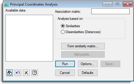
Stats | Multivariate Analysis | Principal Coordinates.
Fill in the fields as required then click Run.

You can set additional Options then after running, you can save the results by clicking Save.

Given a symmetric matrix, A say, with values representing the associations amongst a set of n units, principal coordinates analysis attempts to find a set of points for the n units in a multidimensional space so that the squared distance between the ith and jth points is given by:

d_ij = a_ii + a_jj – 2a_ij

If, for example, A is a similarity matrix then a_ii and a_jj are both equal to 1.0, and so this is equivalent to:

d_ij = 2 (1 – a_ij)

Thus similar units are placed close together and dissimilar units are further apart.

The coordinates generated can be arbitrarily located in space as this will not alter the fitted inter-point distances. By convention, the points are centred to have their mean at the origin, and rotated to principal axes, so that the first r dimensions give the best r dimensional fit.

Association matrix

This specifies the name of the symmetric matrix of associations to be analysed and can be selected from Available data. You can specify either a similarity or distance matrix.

Form similarity matrix

This forms a similarity matrix for input to principal coordinates. You should select this menu if you are starting with raw data variates. This opens the Form Similarity Matrix dialog.

Analysis based on

Specifies whether the analysis is based on a similarity matrix or distance matrix. Whereas similarity matrices can be input directly to the analysis, a dissimilarity (distance) matrix requires preliminary transformation. Selecting dissimilarities will ensure the appropriate transformation is applied to the data.

If B is a distance matrix, so that b_ij gives the observed distance between the i^th and j^th units, then the transformation

A = – B * B / 2

will lead to the analysis generating points with inter-point squared distance

d_ij = a_ii + a_jj – 2a_ij = 0 + 0 – 2 * (- b_ij * b_ij / 2 ) = b_ij²

Therefore the analysis will give points that generate the supplied distances; the first r dimensions of the solution will give the best r-dimensional fit.

Action buttons

Run	Run the analysis.
Cancel	Close the dialog without further changes.
Options	Opens a dialog where additional options and settings can be specified for the analysis.
Defaults	Reset options to the default settings. Clicking the right mouse on this button produces a pop-up menu where you can choose to set the options using the currently stored defaults or the Genstat default settings.
Save	Opens a dialog to specify names of structures to save the results from the analysis.

Action Icons

	Pin	Controls whether to keep the dialog open when you click Run. When the pin is down the dialog will remain open, otherwise when the pin is up the dialog will close.
	Restore	Restore names into edit fields and default settings.
	Clear	Clear all fields and list boxes.
	Help	Open the Help topic for this dialog.