Probit Analysis

Select menu: Stats | Regression Analysis | Probit Analysis

Probit analysis is a way of modelling the relationship between a stimulus, like a drug, and a quantal response (success/failure).

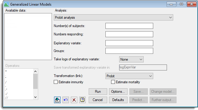
After you have imported your data, from the menu select
Stats | Regression Analysis | Probit Analysis.
Fill in the fields as required then click Run.

You can set additional Options then after running, you can save the results by clicking Save.

It is assumed that for each subject there is a certain level of dose of the stimulus below which it will be unaffected, but above which it will respond. This level of dose, known as its tolerance, will vary from subject to subject within the population. In probit analysis, the tolerance is assumed to follow a Normal distribution, possibly after transforming the doses to logarithms. So, if you were to plot the proportion of the population with each tolerance against (log) dose, you would obtain the familiar bell-shaped curve. Likewise, if you plot the probability that a randomly-selected individual will respond, against the logarithm of dose, you would obtain a sigmoid (S-shaped) curve limited below by zero and above by one.

To make the relationship linear, the y-axis is transformed either to probits or to Normal equivalent deviates. (The probit transformation was originally defined as NED+5, but nowadays they are usually taken to be the same.) The Normal equivalent deviate may be familiar as the transformation that is used to produce “probability” graph paper.

In probit analysis, we are interested in estimating the equation of that line. This can be done by performing an experiment in which there are several sets of subjects, each of which is given a different dose of the stimulus.

Available data

This lists data structures appropriate for the input field which currently has focus. You can double-click a name to enter it in the input field.

Number of subjects

Define the numbers of subjects in each set by entering a variate into this field. This can be selected from the Available data list. Alternatively, if all the sets had the same number of subjects, you can enter a number or scalar into the box.

Numbers responding

The numbers responding in each set is specified by entering a variate into this field; you can enter this by selecting it from the Available data list.

Explanatory variate

Specify the dose given to the subjects in each set by entering a variate into this field. You can transform the data to logarithms (base 10 or base e) using the Take logs of explanatory variate field.

Groups

This can be used to fit a sequence of models to data that are classified into groups. The groups are specified by a factor, which can be selected from the Available data list. The first model to be fitted is a single line, ignoring the groups. Next the model is extended to include a different constant (or intercept) for each group, giving a set of parallel lines one for each group. Then, the final model has both a different constant and a different regression coefficient (or slope) for each group. Graphs and further output from this analysis will display information from the final (full) model.

The Accumulated display setting is particularly useful, producing an accumulated analysis of deviance which lets you assess whether there is evidence of non-parallelism for the lines (the final line in the table, representing the interaction between the explanatory variate and the groups factor); if there is no evidence of non-parallelism, the previous line of the table (representing the main effect of the groups factor) assesses whether different intercepts are needed. If the analysis shows that different intercepts are needed but not different slopes, you can use the DROP directive in command mode to remove the interaction between the explanatory variate and the groups factor.

Take logs of explanatory variate

Provides a list of log transformations that can be used for the dose data. You can select to use a log base 10 or log base e transformation.

Save transformed explanatory variate in

When either a log base 10 or log base e transformation has been selected this option is enabled providing a space to specify the name of an identifier to save the transformed data within.

Transformation (link)

Alternative transformations to the probit link can be selected. Other possibilities are the Logit transformation, logit(P%) = log( P% / (100 – P%)), which is very like the probit but approaching zero (to the left) and one (to the right) rather slower than the probit; and the Complementary log-log transformation ( log( -log(100-P%) ), which is relevant to the “one-hit” model (that is infection processes where just one infected particle is sufficient to cause the response).

Estimate mortality

Sometimes subjects may respond even in the absence of any dose. For example, with some short-lived insects, some would have died from natural causes during the period of the experiment. When this option is selected this natural mortality can be included in the model and estimated.

Estimate immunity

There may be subjects that will not respond, no matter how high the dose. When this option is selected the model will include and estimate a parameter for natural immunity.

Action buttons

Run	Run the analysis.
Cancel	Close the dialog without further changes.
Options	Opens a dialog where additional options and settings can be specified.
Defaults	Reset options to the default settings. Clicking the right mouse on this button produces a shortcut menu where you can choose to set the options using the currently stored defaults or the Genstat default settings.
Save	Opens a dialog where you can save results from the analysis.
Predict	(This option is disabled when probit analysis is selected.) Lets you calculate predictions based on the current regression model.
Change model	This changes the current model by adding or dropping explanatory terms, thus allowing a sequence of models to be fitted and assessed. The Maximal model must be specified to use this option.
Further output	Lets you display additional results and graphical output from the analysis.

Action Icons

	Pin	Controls whether to keep the dialog open when you click Run. When the pin is down the dialog will remain open, otherwise when the pin is up the dialog will close.
	Restore	Restore names into edit fields and default settings.
	Clear	Clear all fields and list boxes.
	Help	Open the Help topic for this dialog.