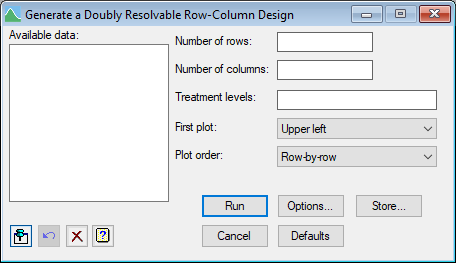
Generate a Doubly Resolvable Row-Column Design

This menu forms approximately optimal doubly resolvable row-column designs using the AFRCRESOLVABLE procedure. Treatments are formed into replicates in both the row and column directions so that the design is doubly resolvable. The layout of plots must be a complete rectangular array, and the treatments must be equally replicated. This requires that the number of rows multiplied by the number of columns in the array must be equal to the number of treatments multiplied by the number of replicates. The row replicates consist of units in adjacent rows, and the column replicates consist of units in adjacent columns. The replicates need not use all plots in a row or column (see the second example below). This design can be thought of as a generalization of a Latin square, with each treatment occurring once in each row and column replicate.

If you have a license for CycDesigN, then the CDNROWCOLUMNDESIGN procedure can be used to produce more efficient designs (but not doubly resolvable ones).

From the menu select
Stats | Design | Generate a Row-Column Design.
Fill in the fields as required then click Run.

You can set additional Options before generating the design.

Two examples

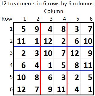
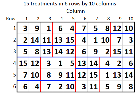
The first design below has 6 rows and columns with 12 treatments in 3 replicates. Each pair of rows makes a row replicate (separated by the blue lines) and each pair of columns (separated by the red lines) makes a column replicate. The second design below has 6 rows and 10 columns with 15 treatments in 4 replicates. A row replicate (separated by the blue lines) contains one and a half rows and the column replicate contains two and a half columns (separated by the red lines).

Analysis of these designs

These designs should be analysed with the Automatic spatial analysis of row-column design menu as, in general, they will not be balanced for fitting row and column replicates in an ANOVA. Balance only occurs where both row and column replicates are made up of complete rows and columns, respectively. This will only happen if the number of rows and columns are both divisors of the number of treatments. For example, the first design above could be analysed with a BLOCKSTRUCTURE of RowReps+ColReps but the second design could not. However, the ANOVA will not fit the row and column effects or spatial trends.

Available data

This lists data structures appropriate to the current input field. It lists either scalars for use in specifying the number of rows, columns or treatments, or variates or texts for specifying the treatment levels. The contents will change as you move from one field to the next. Double-click a name to copy it to the current input field or type the name.

Number of rows

Specify a number or scalar containing the number of rows in the design. This must be between 2 and 4000 with a maximum of 8000 plots in total.

Number of columns

Specify a number or scalar containing the number of columns in the design. This must be between 2 and 4000 with a maximum of 8000 plots in total.

Treatment levels

A number or scalar to specify the number of treatments, or a variate or text to specify the levels or labels of the treatments. The number of levels must be between 2 and 4000. The treatments must be equally replicated, and the number of treatments times the number of replicates must equal the number of plots in the array. The number of replicates (i.e. the number of plots divided by the number of treatments) must be between 2 and 20.

First plot

Specifies where the first plot is located in the array of rows and columns. The rows and columns are always numbered down from the top and across from the left of the array respectively.

Upper left	Plot 1 will be in the upper left of the array, i.e. in the first row and column
Upper right	Plot 1 will be in the upper right of the array, i.e. in the first row and final column
Lower left	Plot 1 will be in the lower left of the array, i.e. in the final row and first column
Lower right	Plot 1 will be in the lower right of the array, i.e. in the final row and column

Plot order

Specifies how the plots are numbered from the first plot and how the plots are allocated to row and column replicates. The rows and columns are always numbered down from the top and across from the left of the array respectively.

Row-by-row	Plots are numbered across the rows, always from the same side
By row in a serpentine way	Plots are numbered in a serpentine/zigzag manner, across a row and then back across the next row and so on, i.e. odd rows are numbered from one side and even rows from the other side
Column-by-column	Plots are numbered along the columns, always from the same end
By column in a serpentine way	Plots are numbered in a serpentine/zigzag manner, along a column and then back along the next column and so on, i.e. odd columns are numbered from one end and even columns from the other end

Options

Opens the Options dialog for choosing which results to display.

Store

Opens the Store Options dialog for choosing which design factors to save.

Action Icons

	Pin	Controls whether to keep the dialog open when you click Run. When the pin is down the dialog will remain open, otherwise when the pin is up the dialog will close.
	Restore	Restore names into edit fields and default settings.
	Clear	Clear all fields and list boxes.
	Help	Open the Help topic for this dialog.