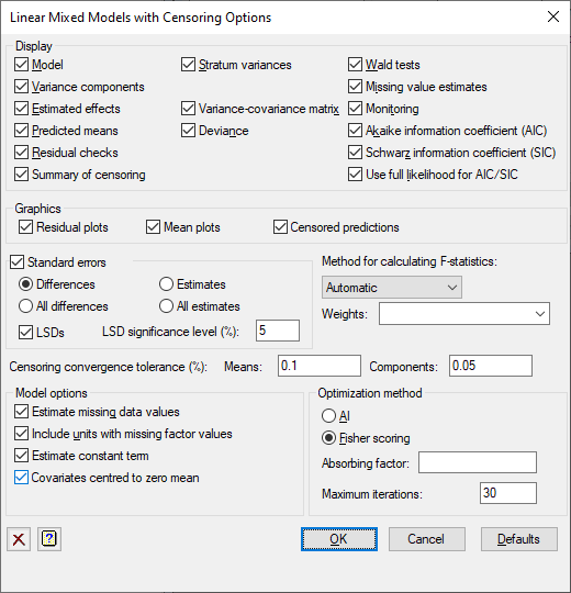
Selects information to be printed by a linear mixed model with censoring analysis and controls certain aspects of the method used.
Display
This specifies which items of output are to be produced by the analysis.
| Model | Description of the model fitted by the analysis |
| Variance components | Estimates of variance parameters |
| Estimated effects | Estimates of regression coefficients |
| Predicted means | Predicted means |
| Residual checks | Uses the VCHECK procedure to check the residuals for outliers and variance stability |
| Summary of censoring | Gives a summary of fitting the predicted values to the censored observations |
| Stratum variances | Estimates of approximate stratum variances |
| Variance-covariance matrix | Variance-covariance matrix for the variance parameters |
| Deviance | The residual deviance |
| Wald tests | Wald Tests for fixed model terms and accompanying F-statistics (if selected) |
| Missing value estimates | Estimates of values missing from the input |
| Monitoring | Monitoring information at each iteration |
| Akaike information coefficient (AIC) | Akaike Information Coefficient to assess the random model |
| Schwarz information coefficient (SIC) | Schwarz Information Coefficient to assess the random model |
| Use full likelihood for AIC/SIC | The information coefficients are calculated using the full log-likelihood from the VKEEP procedure, otherwise the residual log-likelihood is used. See the VAIC procedure for details. |
Graphics
This specifies which graphics are produced by the analysis.
| Residual plots | This gives a default residual plot from the fitted model |
| Means plots | This gives default plot of the predicted means against the factors in the model |
| Censored predictions | This plots the estimated y values against the observed y values |
More control over the residual and mean plots can be obtained by using the Further Output dialog.
Standard errors
Tables of means and effects are accompanied by estimates of standard errors. You can choose whether Genstat computes standard errors or standard errors of differences (SEDs) for the tables. Approximate least significant differences (LSDs) for the predicted means of the fixed terms specified in the Model terms for effects and means field can be computed by selecting LSDs. These are calculated using the approximate numbers of residual degrees of freedom printed by the analysis in the d.d.f column in the table of tests for fixed tests (produced by selecting the Wald tests display option). The degrees of freedom are relevant for assessing the fixed term as a whole, and may vary over the contrasts amongst the means of the term. So the LSDs should be used with caution. If you are interested in a specific comparison, you should set up a 2-level factor to fit this explicitly in the analysis. The significance level for LSDs can be specified as a percentage (default 5) in the accompanying field.
Method for calculating F-statistics
This controls whether Wald tests for fixed effects are accompanied with approximate F statistics and corresponding numbers of residual degrees of freedom. The computations, using the method devised by Kenward & Roger (1997), can be time consuming with large or complicated models. So, the default setting automatic, can be used to allow Genstat to assess the model itself and decide automatically whether to do the computations and which method to use. The other settings allow you to control what to do yourself:
| none | No F statistics are produced |
| algebraic | F statistics are calculated using algebraic derivatives (which may involve large matrix calculations) |
| numerical | F statistics are calculated using numerical derivatives (which require an extra evaluation of the mixed model equations for every variance parameter). |
Weights
A variate of weights can be supplied to give varying influence of each unit on the fit of the model. This would usually correspond to a known pattern of variance of the observations, where the weights would be the reciprocals of the variances. A variate that specifies the weights in the analysis can be selected from the drop down list or you can type its name into the field. If the y-variate has been specified, only variates that match its length will be displayed in the list. The variates in the list are sorted in the standard available-data order.
Censoring convergence tolerance (%)
This controls the convergence criterion of the E-M algorithm in the TOBIT procedure. When the changes between cycles in Means and variance Components are both less than the given percentages, then the algorithm will stop.
Estimate missing data values
This specifies whether predictions are formed from the fitted model for missing values of the y-variate; alternatively any units with missing values in the y-variate are excluded from the analysis.
Include units with missing factor values
This specifies whether data units with missing values in any of the factors in the fixed or random models are included in the analysis. Units with missing y values are always excluded from the analysis.
Estimate constant term
Specifies whether a constant term is included in the fixed model.
Covariates centred to zero mean
Specifies whether covariates are centred to zero mean during the analysis. This applies to all covariates in the model. If covariates are centred, tables of predicted means are based on the mean covariate value, otherwise zero for each covariate.
Optimization method
The AI (Average Information) method is the standard optimization method for REML in Genstat. It uses sparse matrices and is particularly recommended for large datasets and/or complex models. An alternative method is Fisher scoring which, if selected, also allows an absorbing factor to be specified in the model. This can be used to reduce the time or space requirements when fitting large models with many parameters. A more detailed discussion of the use and choice of absorbing factors can be found in the Genstat 5 Reference Manual.
Maximum iterations
This specifies the maximum number of iterations to use to optimize the REML likelihood and in the TOBIT model E-M algorithm.
See also
- Linear Mixed Models with Censoring menu.
- Linear Mixed Models (REML) menu.
- Initial Values for specifying initial gamma.
- Further Output for obtaining additional output after fitting a model.
- Save for saving the results from a REML analysis.
- Save REML results in a spreadsheet.
- Residual Plots for generating plots of residuals.
- Means Plots for generating plots of one- or two-way tables of means.
- REML Predictions menu for forming predictions.
- REML directive for command mode use of REML, with additional options to control the algorithm and for more sophisticated analyses.
- VCOMPONENTS directive for further information about fixed, random, and spline model terms.
- TOBIT procedure.
- VCHECK procedure to check the residuals.
- VKEEP procedure to save results from an REML analysis.
- VAIC procedure to calculate information coefficients.
- VLSD procedure to calculate least significant differences.