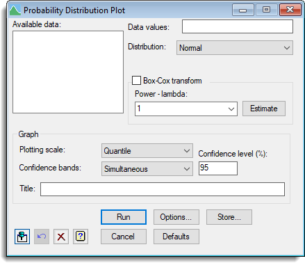
Select menu: Stats | Distributions | Probability Plots
To assess how well empirical data approximates a particular theoretical distribution, the sorted values (order statistics, X(i)) are plotted against the expected values of the order statistics E(i) from the given distribution. However, usually the particular parameters of the distribution are not known and these have to be estimated first to obtain the expected values.
- After you have imported your data, from the menu select
Stats | Distributions | Probability Plots. - Fill in the fields as required then click Run.
You can set additional Options before running and store the results by clicking Store.
If the distribution has a cumulative density function of F(x), and the inverse of this function is G(x) (i.e. G(F(x)) = x), then the expected values of the order statistics, are approximately G((i-0.5)/n), where i = 1…n, and n is the number of values in the sample. A plot of X(i) vs E(i) is known as a Quantile-Quantile (or Q-Q) plot. The data can also be plotted on the probability scale by plotting the cumulative probabilities of the data under the assumed distribution against their expected probabilities, i.e. F(X(i)) vs (i-0.5)/n. This is known as a Probability-Probability (or P-P) plot.
A third plot called the stabilized probability (SP) plot (Michael, 1983), was introduced, which rescales the probabilities using the transformation sp = (2/pi)*arcsin(sqrt(p)), so that the variance of the plotted points are approximately equal over the range of probability values. In the SP plot the scaled values sp are plotted rather than the unscaled p values.
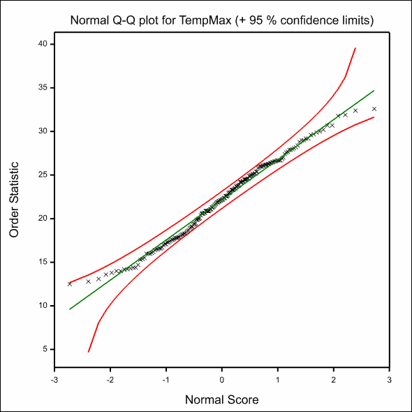
The following graph shows a Normal Q-Q plot with 95% simultaneous confidence bands and a 1-1 reference line.
Available data
This lists variates that are available for analysis. Double-click a name to copy it to the Data values field or type the name.
Data values
This specifies the name of the variate that will be used in the probability distribution plot.
Distribution
This provides a dropdown list of the range of continues distributions that the observed data can be plotted against.
Degrees of freedom
Some of the distributions (Chi-square, t and F) cannot have the parameters estimated by the usual distribution fitting facilities, so these fields provide the degrees to specify the parameters of these distributions.
Box Cox transform
Select this to perform a Box Cox transform on the data before plotting it. The Box Cox transform for a variate X is defined as:
Y = (X**lambda - 1)/lambda	if lambda is not equal to 0, and
Y = LOG(X) 			if lambda = 0.
The power lambda is specified in the field provided.
If X does not have a normal distribution, a value of lambda can often be found such that Y is normally distributed.
For a Normal distribution, the Estimate button will use the YTRANSFORM command to calculate the optimal value of lambda (to the nearest 0.1 between -4 and 4) to transform the X values to a Normal distribution. The optimal value of lambda should be placed in the field above, unless the server is busy with other calculations, in which case you will need to cut and paste the value of lambda from the Output window when the server has completed the calculation.
Plotting scale
The graph can be plotted on three scales:
- Quantile – This plots a Q-Q plot of the observed data values plotted
against their expected quantiles - Probability – This plots a P-P plot of the observed data values
transformed to a probability via the cumulative distribution function of the
theoretical distribution plotted against their expected probabilities - Stabilized probability – This plots the stabilized probability plot of
Michael (1983) described above
Confidence bands
This dropdown list allows two forms of confidence intervals to be displayed in the graph.
- Pointwise simulates distributions of the same size as the data
from the theoretical distribution and plots the range of values at each value
of the order statistics that contain the proportion alpha (specified as a % in
the edit box Conf. Level) of simulated values. Thus a sample drawn from
the assumed distribution has approximately a probability alpha of lying within
the limits at each point. However, overall there will be a probability of less
than alpha that a sample will completely lie within the confidence bands. - Simultaneous uses a statistic given by Michael, 1983, for which the
overall probability of plotted data lying completely within the confidence bands
is approximately the specified value of alpha, under the null hypothesis that
the data are a random sample from the specified distribution. This form of
confidence limits has the advantage that it is much faster to calculate and that
probability of the data points falling outside the limits is approximately
constant over the range of the data. - None specifies no confidence bands to be drawn on the graph.
Action buttons
| Run | Run the analysis. |
| Cancel | Close the dialog without further changes. |
| Options | Opens a dialog where you can specify additional options and settings for the analysis. |
| Defaults | Reset to the default settings. Clicking the right mouse on this button produces a shortcut menu where you can choose to reset using your currently stored defaults or the Genstat default settings. |
| Store | Opens a dialog to specify names of structures to store the results from the analysis. |
Action Icons
| Pin | Controls whether to keep the dialog open when you click Run. When the pin is down |
|
| Restore | Restore names into edit fields and default settings. | |
| Clear | Clear all fields and list boxes. | |
| Help | Open the Help topic for this dialog. |
See also
- Probability Distribution Plot Options
- Probability Distribution Plot Store Options
- DPROBABILITY procedure
- Fit Distribution menu
- Further details of distributions
- Probability Distribution Calculations
- Empirical Distribution Tests
- DPROBABILITY procedure
- DISTRIBUTION directive in command mode
- YTRANSFORM procedure
- EDFTEST procedure
- NORMTEST procedure
- Kernel Density Estimation menu