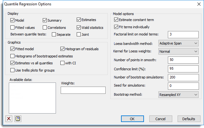
Use this to set the options for the Quantile Regression dialog.
Display
The results to be displayed in the Output window:
| Model | A description of the regression model to be fitted. |
| Summary | A summary of how well the model fitted. |
| Estimates | Estimates of the parameters in the model. |
| Fitted values | Table containing the values of the response variate, the fitted values and residuals from the regression. |
| Correlations | Correlations between the parameter estimates. |
| Wald statistics | The Wald statistics for the separate model terms if Fit terms individually is selected or for the combined model otherwise. This requires bootstrapping to be produced. |
| Between quantile tests | There are two types of test of the significance of the differences between quantiles: Separate – this tests each individual model parameter one by one and Joint – this tests all model parameters jointly. |
Note: Between Quantile tests will produce no output unless multiple quantiles have been specified.
Graphics
The graphs to be produced from the analysis:
| Fitted model | Plot the fitted values vs. the explanatory variate. If groups or a factor are in the model, it will plot the fitted values by group. If multiple explanatory variates are in the model, the first one will be used. |
| Histogram of residuals | Plot a histogram of the residuals for each quantile. If groups are defined, then a trellis histogram for each group will also be produced. |
| Histogram of bootstrapped estimates | Plot a histogram of the bootstrapped estimates for all parameters in the model. |
| Estimates vs. all quantiles | For model parameters, plot the parameter value vs. the quantile with all the distinct quantiles between 0 and 1. |
| with CI | For the above graph, plot confidence limits around the curve. |
| Use trellis plots for groups | For the spline and loess models, if groups are specified then this options will produce fitted value plots in a trellis plot rather than in individual plots for each group. |
Estimate constant term
Whether to estimate a constant as part of the regression model.
Fit terms individually
Whether to separate or pool the information on each term in the Wald statistics. If you pool, for example with A + B, then you will get a single Wald Statistic for A + B, whereas if you don’t pool, then you get separate Wald statistics for A and then B (after fitting A). Obtaining separate Wald statistics takes longer, as the model components are fitted in steps.
Factorial limit on terms
Controls the level of interactions to be fitted. The value entered indicates the level of interaction allowed in the model (that is, set a limit on the maximum number of factors in the interaction terms that are fitted). For example, setting this to 1 will fit only the main effects (1 factor only in fitted terms), and setting this to 2 will only allow first order interactions of the form A.B, and higher order interactions such as A.B.C will not be included in the model. The terms not included in the model will be assigned to the error term.
Loess bandwidth method
How to interpret the loess bandwidth:
| Adaptive span | set the size of the interval around the point to include this proportion of the data. The size of the weighting interval will vary depending on the density of data around the point. |
| Constant width | The interval is a proportion of the range of the explanatory variate and is keep constant for all points. |
Kernel for Loess weights
The weighting function W(d) is for the kernel used in forming the local weights in loess:
| Uniform | W(d) = 1 |
| Linear | W(d) = 1 – ABS(d) |
| Quadratic | W(d) = 1 – d**2 |
| Quartic | W(d) = (1 – d**2)**2 |
| Triweight | W(d) = (1 – d**2)**3 |
| Normal | W(d) = PRNORMAL(d) |
Number of points in smooth
For a spline or Loess model this gives the number of points estimated between the minimum and maximum of explanatory variate that the smooth will be calculated at. Increasing this will increase the time to the the model.
Confidence limit (%)
This gives the probability (as a percentage) that the confidence interval covers the true value. This should be a value between 0 and 100 and if it is too close to 100 then it will not be well estimated unless the number of bootstraps is large.
Number of bootstrap simulations
This gives the number of bootstrap simulations that will be performed to obtain confidence limits, standard errors and estimates of significance. Increasing this increases the time to perform the regression, but produces more precise estimates of the confidence limits etc.
Seed for simulations
This gives a seed to initialize the random number generation used for bootstrapping. Using zero initialises this from the computer’s clock, but specifying an nonzero value gives a repeatable analysis.
Bootstrap method
How to perform bootstraps:
| None | do not do any bootstrapping. |
| Resampled XY | randomly select units with replacement. |
| Weighted XY | randomly weight units with a exponential distribution (only for linear models, not loess or spline models). |
Available data
This lists data structures appropriate for the edit box which currently has focus. You can double-click a name to enter it in the edit box.
Weights
A variate specifying the weights for each of the units in the regression. If field is left blank then equal weights of 1 will be used. This is not available for the spline or loess regression models.
Action buttons
| OK | Save the option settings and close the dialog. |
| Cancel | Close the dialog without making any changes. |
| Defaults | Reset the options to their default settings. |
Action Icons
| Clear | Clear all fields and list boxes. | |
| Help | Open the Help topic for this dialog. |
See also
- Quantile Regression menu
- Quantile Regression Store Options
- Quantile Loess/Spline Regression Store Options
- Nonlinear Quantile Regression menu
- Standard Curves menu
- RQLINEAR procedure
- RQSMOOTH procedure
- RQNONLINEAR procedure
- FRQUANTILES directive
- RQOBJECTIVE function