Nine slides were produced using an Affymetrix Arabidopis chip (ATH1-121501) with 22810 probes arranged in a 712 x 712 grid. Arabidopis is a simple plant often used in gene studies. The CEL file data for these chips are stored in the files hyb1191.CEL-hyb11400.CEL and the layout of probes and quality control units can be found in the CDF file ATH1-121501B.CDF. The 9 slides have three replicates of three targets applied to them.
Import the example data
These example data files can be found in this downloadable file Microarrays.zip. These should then be unzipped to the folder C:\Program Files\GenxxEd\Data. (Replace ‘xx‘ with your Genstat version number e.g. ‘Gen21Ed’. This will create a Microarrays folder under Data).
If you do not have rights to unzip files to that directory, then they can be placed in any directory, but will not be found in the File | Open Example Data Sets menu.
If you are unsure of how to unzip the files, then opening the Microarrays.zip file with File | Open will let you select a file from the zip file.
Calculate expression values
To calculate expression values for these 9 slides, we first need to open the files. The CEL and CDF files can be opened individually using the menu File>Open. You can also open files from the menu by selecting Stats>Microarrays>Data>Affymetrix CEL Files as shown below:

To select the CEL files click on the browse button ![]() and select all the files as shown below:
and select all the files as shown below:


The CEL files will be opened in the order that the files appear in the list. Use the Up and Down buttons to rearrange the order of the CEL files within the list.
Once the CEL files have been selected the corresponding CDF file can be selected by clicking the Browse button ![]() adjacent to the CDF file field and selecting the file ATH1-121501B.CDF. Selecting this file will result in the completed menu shown below.
adjacent to the CDF file field and selecting the file ATH1-121501B.CDF. Selecting this file will result in the completed menu shown below.

Clicking Open will display the following menu
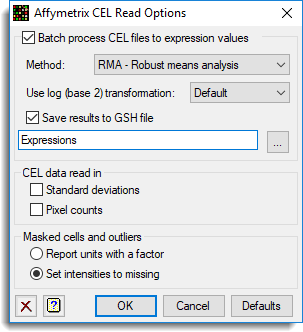
Select the option for batch processing with the RMA method, and provide the filename, Expressions.gsh, to save the results. Note, this analysis can be very slow, as each CEL file contains over half a million observations. However, the results for the batch processing can be found in the Genstat spreadsheet file Hyb-Expressions.gsh in the the downloadable Microarrays.zip file.
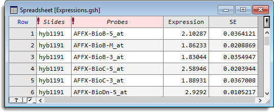
Opening the CEL files or opening the file Hyb-Expressions.gsh will produce a spreadsheet containing the following columns:
Opening the Expressions.gsh spreadsheet that was saved to your working directory produces a spreadsheet containing the following columns.
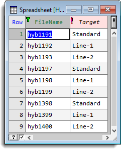
The data can be summarized using a single channel analysis of variance. Before the analysis can be performed the structure of the targets applied to the slides is required. This structure can be found in the file HybFiles.gsh. To open this file select File | Open and navigate to the same location where you found the .CEL files, then select the file HybFiles.gsh and click Open.
This will open the spreadsheet shown below.
Now, to summarize the data select Stats>Microarrays>Analyse>One Channel ANOVA. The image below shows the menu with the data names entered in the fields.

To estimate the difference between the standard treatment and the other two cell lines, we can specify a contrast, by clicking on the Contrasts button. This opens the following menu:

Here we have selected the Target factor for the contrasts factor, set the number of contrasts to 2 and the comparisons contrast type. Clicking OK creates a blank matrix spreadsheet with 2 rows and 3 columns where the values for the contrasts can be entered. In this matrix (see below) we have entered 2 contrasts; the first compares line 1 vs the standard and the second line 2 vs the standard.

Returning to the single channel ANOVA menu, we now set additional options and specify the names of structures to save the results into. Clicking on the Options button opens the menu shown below. Here we have left the options at their default settings.

The results from the analysis can be stored when the analysis is run. To store the results the names of the structures to save the results need to be supplied before running the analysis. To do this click the Store button. This opens the menu below where you can specify the items to be saved. The options at the bottom of the dialog can be used to control whether the results are to be displayed into spreadsheets.

Returning to the one channel ANOVA menu and clicking Run produces an analysis of variance for each probe and displays the stored results in a spreadsheet (as shown below). This may take some time to appear.
An alternative way to analyse this data would be to use the Robust Means Analysis menu. To access this select Stats>Microarrays>Analyse>Robust Means Analysis. The image below shows the menu with the fields entered to perform the analysis.

Similar to the single channel analysis of variance menu, options can be set for this menu by clicking the Options button. The image below shows the default options set for a robust means analysis.

See also
- Two channel microarray example
- Single Channel ANOVA menu
- Robust Means Analysis menu
- Microarray Menus
- Histograms,
spatial plots and 2D plots
for visualizing microarray data