Select menu: Stats | Microarrays | Explore | Spatial Plots
Use this to produce a shade plot to display any spatial variation. You can display separate plots for all slides or alternatively from just a subset of these.
- After you have imported your data, from the menu select
Stats | Microarrays | Explore | Spatial Plots. - Fill in the fields as required then click Run.
You can set additional Options before generating the graph.
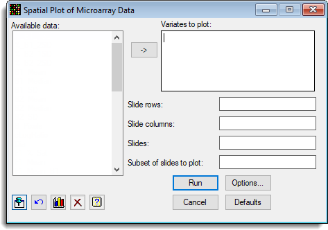
Available data
This lists data structures appropriate for the field which currently has focus. You can double-click a name to enter it in the currently selected field or type the name.
Variates to plot
A list of the variates to be plotted. You can transfer multiple selections from Available data by holding the Ctrl key on your keyboard while selecting items, then click ![]() to move them all across in one action. You can use the usual edit functions and keys to add, delete and change names in this list.
to move them all across in one action. You can use the usual edit functions and keys to add, delete and change names in this list.
Slide rows
A factor that indexes the rows across the whole slide.
Slide columns
A factor that indexes the columns across the whole slide.
Slides
The factor that identifies the slides. If just a single slide is being displayed you do not need to provide this.
Subset of slides to plot
Lets you specify a subset of the slides from the data set to be plotted. To plot a subset of slides you can specify a list of the levels or labels of the slides factor. For a list of factor levels or labels the numbers or labels should be separated by either spaces or commas. Note that for a list of factor labels where one or more of labels contain a non-alphanumeric character (space, -, + etc…) in the name the label(s) must be specified within single quotes. For example, ‘MS 1′,’MS-2’, ‘MS+3’.
Action buttons
| Run | Generate the graphs. |
| Cancel | Close the dialog without further changes. |
| Options | Opens a dialog where additional options and settings can be specified for the graphs. |
| Defaults | Reset options to their default settings. Clicking the right mouse on this button produces a shortcut menu where you can choose to set the options using the currently stored defaults or the Genstat default settings. |
Action Icons
| Pin | Controls whether to keep the dialog open when you click Run. When the pin is up |
|
| Restore | Restore names into edit fields and default settings. | |
| Graphics Output | Controls how graphs are to be drawn. You can either draw the graph in the Graphics View or save direct to files (JPEG, TIFF, EPS, EMF, GMF, BMP or PNG). | |
| Clear | Clear all fields and list boxes. | |
| Help | Open the Help topic for this dialog. |
Example
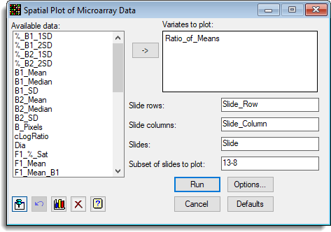
The following dialog shows the plotting of a the log-ratios of a single slide (Data13-6-9.gwb).
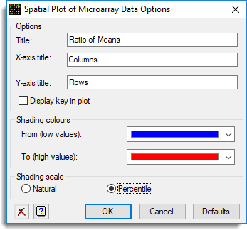
The graph titles and colours where set using the Spatial Plot Options dialog.
This is the resulting graph:
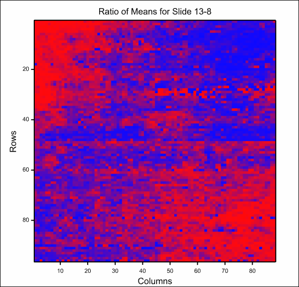
High values are shown in red, low values in blue and mid range values in the mix of blue and red are purple. Missing values are displayed in black.
See also
- Spatial Plot Options
- Microarray Menus
- Histograms, density plots, and 2D plots for other ways of visualizing microarray data
- Two Channel Microarray Example
- Microarray procedures
- MASHADE procedure
- DSHADE directive