Select menu: Stats | Microarrays | Analyse | False Discovery Rate using Bonferroni
Use this to estimate false discovery rates (defined in the table below) using a Bonferroni-type procedure.
- After you have imported your data, from the menu select
Stats | Microarrays | Analyse | False Discovery Rate by Bonferroni. - Fill in the fields as required then click Run.
You can set additional Options before running and store the results by clicking Store.
This is a non-parametric approach, where for each value of lambda, the observed proportion of the sample that is not differentially expressed (π0) is calculated. The procedure uses two methods to get an overall measure of π0. The first uses bootstrapping to choose the value of π0 which minimizes the mean squared error, and the second uses a spline smoother to smooth the values of π0 around the maximum value of lambda. Unadjusted q-values are then calculated from the estimate of π0 as π0*p*(Proportion of tests < p) (where p is the test probability) for each test value, and then the Bonferroni q values are defined as the minimum of the q values above each test value, stepping this procedure down through the sorted p values.
The following table defines some random variables related to m hypothesis tests:
| Significance test | # declared non-significant | # declared significant | Total |
| # true null hypotheses | U | V | m0 |
| # non-true null hypotheses | T | S | m1 = m − m0 |
| Total | W = m − R | R | m |
m0 is the number of true null hypotheses
m − m0 is the number of false null hypotheses
U is the number of true negatives
V is the number of false positives
T is the number of false negatives
S is the number of true positives
H1…Hm are the null hypotheses being tested
In m hypothesis tests of which m0 are true null hypotheses, R is an observable random variable, and S, T, U, and V are unobservable random variables.
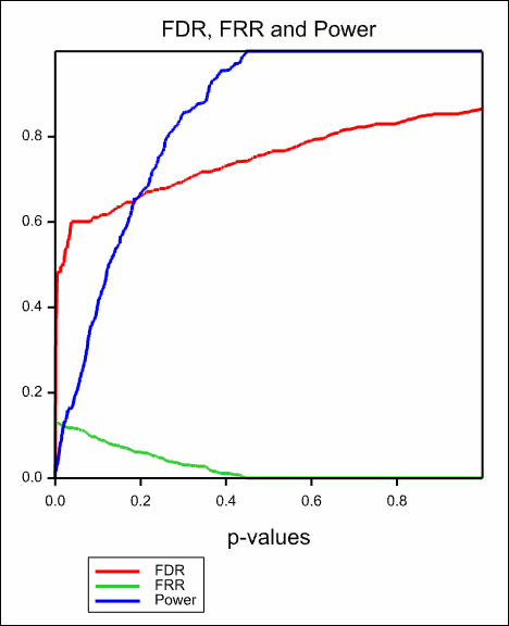
The proportion of tests that are truly null, π0, is m0 divided by m. The false discovery rate (FDR), also known as the q-value of a test, is a commonly used error measure in multiple-hypotheses, defined as FDR = E(V/R | R > 0) × Pr(R > 0), i.e. the expected proportion of false positives findings among all the rejected hypotheses multiplied by the probability of making at least one rejection; the FDR is zero when R = 0. Similarly the false rejection rate (FRR) is defined as FDR = E(T/W | W > 0) × Pr(W > 0), i.e. the expected proportion of false negatives findings among all the accepted hypotheses times the probability of accepting at least one test. We also define the power to be equal to E(S/m1 | m1 > 0) × Pr(m1 > 0).
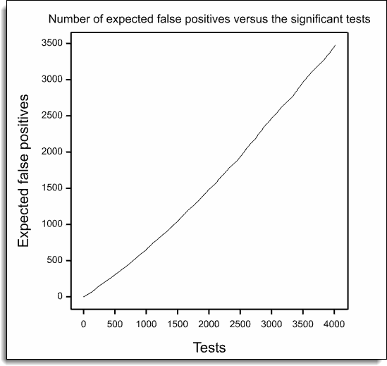
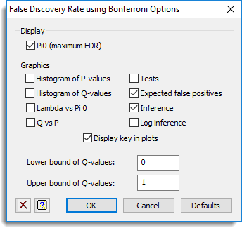
A range of graphs can be plotted after the Bonferroni procedure has been used.
Available data
This lists data structures appropriate for the field which currently has focus. You can double-click a name to enter it in the field or type the name.
Method
Controls the method used for calculating π0:
| Spline smoother | Fits a smoothing spline of λ onto initial estimates of π0 calculated as for a single λ value, and takes the estimate of π0 as the value corresponding to the largest value of λ |
| Bootstrap | Estimates π0 by bootstrap sampling from the variate of p-values. |
Probabilities to model
This variate contains the probabilities to which the mixture distribution is fitted. All the values in the variate should be between 0 and 1 (although missing values (*) are allowed).
Lambda
The tuning parameter λ to be used (scalar or variate). The default is a variate containing the numbers 0, 0.05, … 0.9. λ can be thought of as the value beyond which the individual p-values are considered null. As λ gets larger the bias of π0 gets smaller, but its variance increases. If you set λ to a scalar, π0 is estimated by dividing the number of null tests (i.e. the number of p-values greater than λ) by the expected number of null tests m × (1 – λ). If λ is set to a variate of values, then π0 is estimated at each value of the variate and the resulting values combined according to the method (spline smoother or bootstrap) selected above.
Spline d.f.
Specifies the degrees of freedom to use for the smoothing spline. This should be an integer between 1 and 99.
Use logged Pi 0 values when smoothing
When selected a smoothing spline will be fitted to the log-transformed π0 values.
Action buttons
| Run | Run the analysis. |
| Cancel | Close the dialog without further changes. |
| Options | Opens a dialog where additional options and settings can be specified for the analysis. |
| Defaults | Reset the options back to their default settings. Clicking the right mouse on this button produces a pop-up menu where you can choose to set the options using the currently stored defaults or the Genstat default settings. |
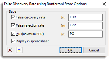
| Store | Opens a dialog to specify names of structures to store the results from the analysis. The names to save the structures must be supplied before running the analysis. |
Action Icons
| Pin | Controls whether to keep the dialog open when you click Run. When the pin is down |
|
| Restore | Restore names into edit fields and default settings. | |
| Clear | Clear all fields and list boxes. | |
| Help | Open the Help topic for this dialog. |
Example
The following image shows the estimates of FDR using the Bonferroni procedure (ApoAIKnockOutEffects.GSH).
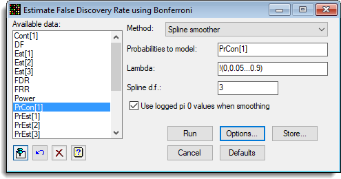
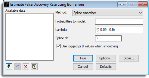
The options used were:
and the Store button was used to save results back to a spreadsheet:
The resulting graphs are show below: