Normalize Two Channel Microarray data

Select menu: Stats | Microarrays | Normalize | Two Channel

For large arrays it is essential to identify sources of variation and correct for them to allow for robust use of this technology. Through normalization procedures, such variations can be identified and removed to obtain data for follow on research.

The sorts of spatial artifacts removed from a slide can be seen in a spatial plot.

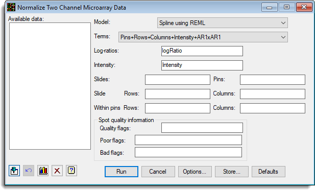
After you have imported your data, from the menu select
Stats | Microarrays | Normalize | Two Channel.
Fill in the fields as required then click Run.

You can set additional Options before running the analysis and store the results by clicking Store.

The analysis of the microarrays is a two-step analysis; with a within slide analysis aimed at normalization and if required standardisation, and then a between slide analysis to estimate the differences between targets, and their consistency. Various techniques for normalisation have been suggested, including linear regression, ratio statistics, local smoothing and analysis of variance. The approach used in this menu is to model the variation associated with spatial and structural components and remove this as noise. Examples of spatial components are the grid layout on the slide (rows x columns), and of structural components are the pins, print order and differential dye responses to binding and scanning. The model can be specified to fit the type of variation found in the particular series of slides. The usual statistical modelling approach is taken where all possible sources of noise are jointly fitted in one model, with the need for each term being assessed using statistical significance of the reduction in remaining unexplained variation. Model terms can be added or removed as required. The fitted model then indicates where useful modification of protocols and equipment would help minimise variation in future experiments.

Available data

This lists data structures appropriate for the field which currently has focus. You can double-click a name to enter it in the currently selected field or type the name.

Model

Two types of model can be used to normalize the data:

Spline using REML – Mixed model using cubic smoothing splines fitted with the REML directive.
Loess using FIT – Regression using the LOESS smoothing function.

Terms

The model terms to fit to the log-ratios. Select the model that you want to fit from the dropdown list. The terms are made up of the following components:

Pins – A separate mean for each pin on the slide.

Rows – A separate mean for each row on the slide.
Columns – A separate mean for each column on the slide.
Intensity – A cubic smoothing spline or Loess curve (maximum degrees of freedom set in the options menu)
for spot intensity.
AR1 – an autoregressive model with order 1, separately in row and columns (REML only)
Spline(Row.Column) – A thin-plate spline which fits a smooth surface with row and
column interaction
(REML only)

The selection of terms will enable or disable the fields below required to fit the model. For the AR1 term, the Within pins rows and columns are required. For the Row and Column terms, the whole slide rows and columns terms are required respectively.

Log-ratios

The log-ratios (generally calculated using the calculate microarray log-ratios menu) to normalize.

Intensity

The brightness of the spot on the log scale, usually calculated with the calculate microarray log-ratios menu. If the Intensity term is not being fitted you do not need to provide this.

Slides

The factor that identifies the slides. If just a single slide is being normalised you do not need to provide this.

Pins

A factor that indexes the print groups or pins that printed the spot within each slide. Pins may deliver different aliquots of DNA when printing the spots, or may become blocked and so change the level of the log-ratio for that group of spots on the slide. As pins generally print adjacent spots, pin effects will also be confounded with other general spatial effects. If the Pins term is not being fitted you do not need to provide this.

Slide rows

A factor that indexes the rows across the whole slide. Spatial effects may cause variations along the rows. If the Rows term is not being fitted you do not need to provide this.

Slide columns

A factor that indexes the columns across the whole slide. Spatial effects may cause variations along the columns. If the Columns term is not being fitted you do not need to provide this.

Within pin rows

A factor that indexes the rows within the pins. The rows with in each pin should be numbered from 1 to n. This is required to efficiently fit the AR1 autocorrelation along rows. If the AR1 term is not being fitted you do not need to provide this.

Within pin columns

A factor that indexes the columns within the pins. The columns with in each pin should be numbered from 1 to n. This is required to efficiently fit the AR1 autocorrelation along columns. If the AR1 term is not being fitted you do not need to provide this.

Quality flags

The name of the variate or factor that specifies spot quality. Many image analysis systems create a code for the quality of the spots. For example, GenePix creates a variate named Flags that has values -25, and -50 for low intensity spots which it regards a poor quality and values of -75 and -100 for spots that have bad quality due scratches or other image artifacts or intervention by the user to mark them as bad.

Poor flags

The codes in the Quality flags structure that indicate poor quality spots. Poor quality spot information is used for the normalization process, but the corrected log-ratios are returned as missing. For example, GenePix uses values -25, and -50 to mark poor quality spots.

Bad flags

The codes in the Quality flags structure that indicate bad quality spots. Bad quality spot information is not used for the normalization process and the corrected log-ratios are returned as missing. For example, GenePix uses values -75, and -100 to mark poor quality spots.

Action buttons

Run	Run the analysis.
Cancel	Close the dialog without further changes.
Options	Opens a dialog where additional options and settings can be specified for the analysis.
Defaults	Reset options to their default settings. Clicking the right mouse on this button produces a shortcut menu where you can choose to set the options using the currently stored defaults or the Genstat default settings.
Store	Opens a window to specify names of structures to store the results from the analysis. The names to save the structures must be supplied before running the analysis.

Action Icons

	Pin	Controls whether to keep the dialog open when you click Run. When the pin is up the dialog will remain open, otherwise when the pin is down the dialog will close.
	Restore	Restore names into edit fields and default settings.
	Graphics Output	Controls how graphs are to be drawn. You can either draw the graph in the Graphics View or save direct to files (JPEG, TIFF, EPS, EMF, GMF, BMP or PNG).
	Clear	Clear all fields and list boxes.
	Help	Open the Help topic for this dialog.

Example

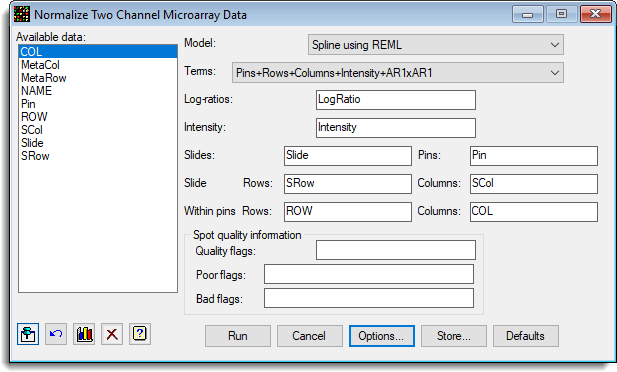
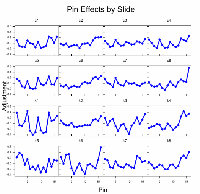
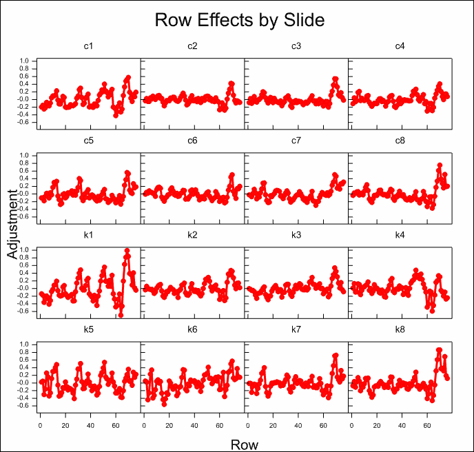
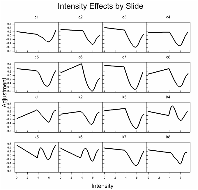
The following example shows the Normalization of a mouse knock out experiment with 6384 genes per slide. There were 16 slides in this experiment, 8 control mice and 8 knock out mice all on the red dye compared to a standard reference on the green dye. The normalization fits pin, row and column effects and dye intensity effects. The estimated effects for these can be seen in the following plots produced by the procedure. The menu settings used to normalize this data are shown here:

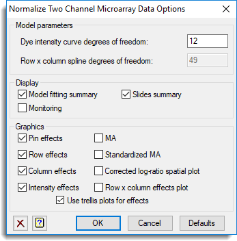
The options to set the spline degrees of freedom and the plots/display to produce were set in the Options dialog. The graphs for the different effects have been selected to be displayed for each slide within trellis plots.

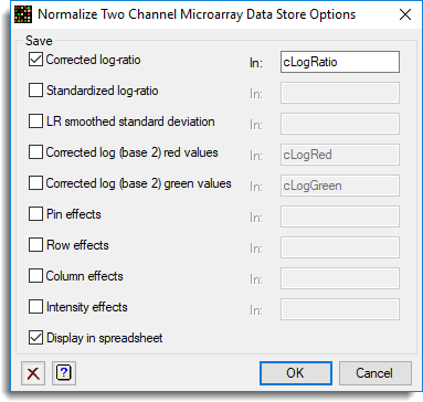
Just the corrected log-ratios were saved and added back to the originating spreadsheet.

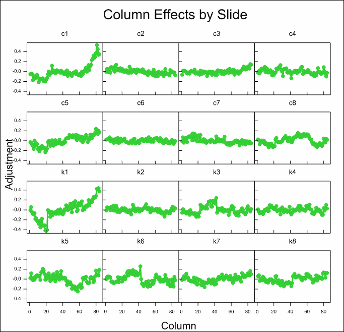
The estimated effects of the various model components are displayed for all slides in the following trellis plots. It can be seen that there are large effects for most of the components. The normalization model explains over 50% of the variation on the slides.

The column effects on most slides are small, with the exception of the first control and knock out slides c1 and k1 where there is a strong trend on one side of the slides.