Select menu: Spread | New | Append Multiple Excel Worksheets
Use this to append data from one Excel file containing multiple sheets into a single spreadsheet. The new spreadsheet created from the appended data includes a factor, with the column name WorkSheet, that indexes the worksheet source from where the data were opened from. The name of each appended worksheet is used for the labels for each group of this indexing factor.
- From the menu select Spread | New | Append Multiple Excel Worksheets.
- Navigate to your Excel file then select it and click Open to display the dialog below.
- In the Select multiple sheets/ranges list select the items you want to append. Hold down Ctrl or Shift as you click to select more than one item
- In the Add to book dropdown list select the book or spreadsheet to append the new data to or leave this set to New book to create a new book from your selections.
- Set other options as required then click OK.
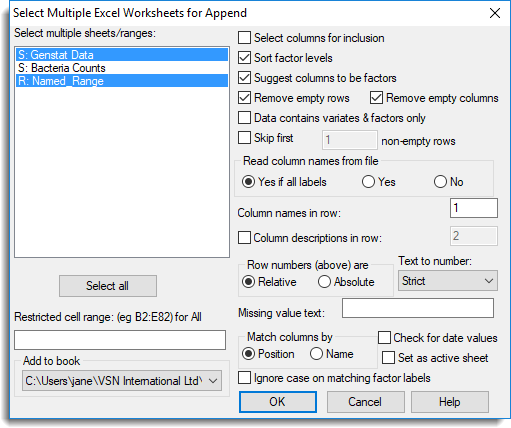
The dialog above shows one sheet and one named range have been selected to add to an existing book.
Select multiple sheets/ranges
Select one or more sheet names to read the data from. By default only one block of data can be opened from a worksheet. However, you can open multiple blocks of data from a single worksheet by creating named ranges. Named ranges have the advantage that both the sheet and cell range are specified permanently in the Excel file, and these are automatically updated if further rows or columns are inserted into the cell range. See Setting up Excel Named Ranges for details on creating a named range in Excel.
Worksheets and named ranges are identified in the list by the prefix S: and R: respectively. By default, if the first row loaded contains text values these will be used as column names in each spreadsheet, otherwise default column names will be generated (this behaviour can be modified using the options below).
Column names ending in an exclamation mark (!) will have this character removed and the column will be loaded as a factor. Likewise names ending with a dollar ($) or a hash (#) will be loaded as text or variates respectively.
The initial format of data can be specified by appending characters to the end of the column name.
- A suffix of :0, :1, :2 … :9 specifies the column is displayed with the given fixed number of decimal places.
- A suffix of :E specifies the column is to be displayed in scientific format.
- A suffix of :D specifies the column is to be displayed in date format. The actual format to display the date will be the default date format for Genstat.
- A suffix of :T specifies the column is to be displayed in time format.
Characters in column names that are invalid for Genstat identifier names are converted to underscore (_).
Factor levels, labels and their order can be supplied in Excel by adding a comment to the cell containing the column name. The factor labels or levels must start with a ! on a new line in the comment. To provide levels use the format !(100,90,50,10). Alternatively, to provide labels use the format !T(Control,A,B,C) or !t(‘Control’,’A’,’B’,’C’). The order of the items in the comment will define the order of the levels or labels in the factor. If a column in Excel just contains ordinal values (i.e. 1…n), the comment can still be used to assign labels or levels to these groups. The first item in the comment will define the level or label for group 1 in the factor etc.
Column description information can also be supplied in the comment, and is specified by any line of text not starting with an exclamation mark.
The following image shows two comments entered into Excel (use the Excel menu item Insert | Comment to do this, making sure you do not put any line breaks in the middle of the list).

More information on this can be found in Using Genstat with Excel.
Restricted cell range
If specified, the same cell range is used on each sheet as within the Excel file. However, you can load a subset of the data from a worksheet by specifying the position of diagonally opposite corners of the rectangle that spans the required range. For example, the range B12:E18 will load seven rows and five columns starting at row 12 of the second column (B).
The range can also be specified by using partial column or row information as follows:
- Just the starting cell can be given (e.g. B12) and all cells to the lower right will be used.
- Just column letters provided (e.g. B:E), and all rows in these columns will be used.
- Just row numbers provided (e.g. 12:18), and all columns with data in these rows will be used.
Select columns for Inclusion
Lets you select a subset of columns from the worksheet. This opens the Select Columns dialog once the data has been read in.
Sort factor levels
When selected, columns loaded as factors will have their levels (or labels for a text column) sorted into ascending order.
Suggest columns to be factors
Prompts to convert columns to factors where the columns have repeated values, and fewer unique values than the specified number given in the Suggest converting columns with <= N unique items option within the Tools | Spreadsheet Options | Conversions tab.
Remove empty rows
Remove any rows from the spreadsheet that only contain missing data.
Remove empty columns
Keep any empty columns from the spreadsheet. The default behaviour is to only include columns that contain data.
Data contains variates & factors only
Any column containing text will be converted to either a variate or factor. If the number of rows containing labels within the spreadsheet column is less than 20%, the column will be converted into a variate, otherwise the column will be converted into a factor. When reading the column as a variate, common typing errors such as entering a letter O for the number 0 (or I for 1) will be fixed.
Skip first X non empty rows
Skip the first specified number of rows before reading the data. Often at the start of a spreadsheet there are some comments and this option can be used to skip over these. Labels in these rows can still be used in either the names or extra components of a column.
Read column names from file
Specifies whether to read the column names from the file.
| Yes if all labels | The names will be read from the row specified in the names row (below) if all the cells in this row contain only labels or are missing. A default column name will be generated for a missing cell. |
| Yes | Use the cells in the name row for column names. If the cell contains a number prefix this with a “_” to make it a valid Genstat name. |
| No | Do not read the names from the file and generate all default names. |
Column names in row
The row number (within the selected range) to use for column names. A row number within the skipped rows may be used if required.
Column descriptions in row
If this option is checked, the cells in the specified row number (within the selected range) will be used for column descriptions (the EXTRA keyword for Genstat structures). A row number within the skipped rows may be used if required.
Row numbers
| Relative | Taken from the top of the restricted cell range. |
| Absolute | Taken from the top of the spreadsheet and thus correspond to the absolute row numbering in Excel/Quattro. |
Text to number conversions
This controls how labels are interpreted as numbers when a label is forced to be an entry in a variate:
| Strict | Only labels that contain numeric data only are converted (e.g. ’10’ -> 10, ‘1O’ -> *.) |
| Single | A single character substitution is read as a number (o,O -> 0, i,I,l,L -> 1, s,S-> 2, z,Z -> 5, comma -> decimal point) (e.g. ‘1O’ -> 10, ‘Io’ -> *). |
| Common | Mmultiple substitutions as in single are made (e.g. ‘Io’ -> 10, ’23X’ -> *). |
| Standard | As in common but extra text is ignored at the end of the number (e.g. ’23X’ -> 23, ‘A2X3’ -> *). |
| Lax | Any digits are read from the text (e.g. ‘A2X3’ -> 23). |
Missing value text
By default, empty cells or cells with a text consisting of a single asterisk * are read in as missing values (unless the column is a text column, in which case the * is read in as a text value ‘*’). If an alternative string to * has been used as a missing value place holder in the worksheet then entering this text here will cause this to be interpreted as a missing value in numerical columns. For example, a user may have entered ‘M’ for a missing value or may have added a note ‘Died’ in a column of live weights.
Match columns by
| Position | Data from column 1 will be appended to column 1, 2 to 2 etc. |
| Name | Data from columns with the same name will be appended to each other. |
Add to book
This lists all open books within Genstat. Select the book that the new sheet will be added to. If the data are to appear in a new book then select the New book setting.
Check columns for date values
When selected, Genstat checks all text columns to see if they contain data in date format. If columns appear to contain data in date format you are prompted to convert these to date values. The default setting for the this option can be set on the Tools | Spreadsheet Options | Conversions tab.
Set as active sheet
This sets the new spreadsheet that is created as the Active spreadsheet. See Setting an Active Spreadsheet for more details.
Ignore case on matching factor labels
If this is selected, then when matching factor labels between the existing factor and the appended factor, the case of the labels will be ignored. For example, if one factor had labels A,B,C and the other factor had labels a,b,d then if case was ignored the new factor would have labels A,B,C,d and A,B,C,a,b,d if the case was taken into account on matching.
Action buttons
| OK | Append the sheets and close the dialog. |
| Cancel | Close the dialog without further changes. |
| Select all | Select all items in the Select multiple sheets/ranges list. |
See also
- Spreadsheet New Menu
- Append Multiple Files
- Append Data to Spreadsheet
- Select Worksheet
- Excel Import Wizard
- Using Genstat with Excel
- Setting up Excel Named Ranges
- Spreadsheet File Options Tab
- Understanding Factors within a Spreadsheet
- Options – Date Format
- Merge Spreadsheet
- Spreadsheet Manipulate Menu
- Merge Multiple Files
- Fill Empty Factor Cells in Columns dialog
- Select Columns to be Factors dialog
The APPEND procedure can be used in the command language to append data sets.