
Select menu: Stats | Regression Analysis | Quantile Regression
Use this to fit a quantile regression.
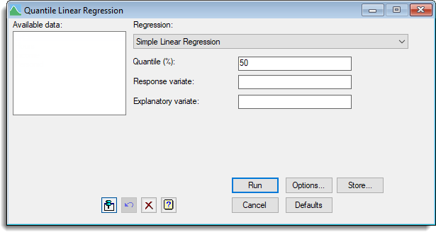
- After you have imported your data, from the menu select
Stats | Regression Analysis | Quantile Regression. - Fill in the fields as required then click Run.
You can set additional Options before running the analysis and store the results by clicking Store.
A quantile regression is the function that minimises the expected absolute loss SUM(e*(Q – (e < 0))) and estimates the Qth quantile of the minimised residuals; where e = Y – Xβ, Q is the quantile between 0 and 1, e are the model residuals, X is the design matrix and β is the coefficients of the model. The Qth quantile is the value which has a proportion Q of the distribution below it. Roughly speaking, the quantile regression can be thought of as the best fitting function that has a proportion Q of the residuals below it. A range of linear functions can be fitted with in this menu covering all the functions that can be fitted with the Linear Regression menu.
The analysis for the menu is performed using the RQLINEAR procedure for all models except the Loess or Spline models for which RQSMOOTH is used.
The output, graphs produced and options controlling the estimation of standard errors by bootstrapping can be changed using the Options dialog which can be opened by clicking on the Options button. The results can be saved into structures by specifying the identifier names using the store dialog which can be opened by clicking on the Store button.
Available data
This lists data structures appropriate for the input field which currently has focus. You can double-click a name to enter it in the input field.
Regression model
This specifies the type of model to be fitted to the response variate. When a model is selected the fields will change on the menu for the appropriate model. The choices of model are:
- Simple Linear Regression
- Simple Linear Regression (with Groups)
- Multiple Linear Regression
- Multiple Linear Regression (with Groups)
- General Linear Regression
- Polynomial Regression
- Smoothing Spline
- Locally Weighted Regression (Loess)
Quantile (%)
Percentages at which to calculate quantiles; default 50%. To fit a number of quantiles, enter a list of values separated by spaces or commas. A variate may also be selected for this in which case quantiles will be fitted for all the values in the variate.
Response variate
A variate containing the y-variate to be analysed. The model Xβ will be optimised to obtain the best fit to this variate.
Model to be fitted
For General Linear Regression, this gives the model to be fitted by entering a model formula. The formula can involve both variates and factors which can be selected from the Available data list, and operators from the Operators list. A variate in the formula represents its linear effect, and a factor represents its main effect: that is, a separate intercept for each level of the factor.
An interaction between factors allows separate intercepts for each combination of levels of the factors. An interaction between a variate and a factor represents separate slopes for each level. You can also include interactions between variates, representing the linear effect of the product of the two variates, and interactions between any number up to nine variates and factors.
There are functions available in the Operators list that provide more general effects of variates than simply the linear effect. The POL() function represents polynomial effects up to the order given in the second argument (maximum 4); so POL(x; 3) represents a cubic effect of the variate x. The POL function cannot be combined in interaction terms, but the S function may appear in interactions with factors, when the linear effect of the variate is estimated separately for each level together with a single smoothed effect for all levels.
Groups
For models with groups this specifies a factor for which separate models are fitted, depending on the choice of the Final model option.
For an analysis of parallelism the first model to be fitted is a simple linear regression, ignoring the groups. Next the model is extended to include a different constant (or intercept) for each group, giving a set of parallel lines one for each group. Then, the final model has both a different constant and a different regression coefficient (or slope) for each group. The list adjacent to the Groups field lets you select between the types of regression model that you want to fit.
Final model
For an analysis of parallelism, if the analysis shows that different intercepts are needed but not different slopes, you can use this option to select the final model and re-run the analysis to remove the interaction between the explanatory variate and the groups factor. Similarly, if different intercepts are not needed this option can be used to fit just the explanatory variate.
Degrees of freedom
For a polynomial model, this is a dropdown list of a linear, quadratic, cubic or quartic model. The higher order models have more flexibility in fitting the data, but use more degrees of freedom.
For a spline this specifies the degrees of freedom to control the smoothness of the spline. This is effectively increasing or relaxing the constraints on the spline, with a higher number allowing more flexibility in the curve fitted to the data.
Bandwidth
This specifies a number between 0 and 1 which indicates the proportion of the data to include in the Locally weighted regression around the point that the model is estimating. As this value decreases the model becomes more flexible and responsive, following individual points, but consequently becomes rougher, more variable and with wider confidence limits. As the value approaches 1 the model becomes smoother and closer to a single model fit using the linear or quadratic function selected by the Polynomial model option below.
Polynomial model
For a Locally weighted regression this specifies the polynomial model to be used for the local fits. You can choose either linear or quadratic.
Operators
This provides a quick way of entering operators in the regression model formula. Double-click on the required symbol to copy it to the current input field. You can also type in operators directly. See model formula for a description of each operator.
Action buttons
| Run | Run the analysis. |
| Cancel | Close the dialog without further changes. |
| Options | Opens a dialog where additional options and settings can be specified for the analysis. |
| Defaults | Reset options to the default settings. Clicking the right mouse on this button produces a pop-up menu where you can choose to set the options using the currently stored defaults or the Genstat default settings. |
| Store | Opens a dialog to specify names of structures to store the results from the analysis. The names to save the structures should be supplied before running the analysis. |
Example 1
The dataset ‘Engel.gsh‘ from the Genstat Examples directory contains the results of a survey of 235 Belgian working class households by Engel in 1857.
- From the menu select File | Open then navigate to the Windows default installation folder C:\Program Files\GenXXEd\Examples and select Engel.gsh.
- From the menu select Stats | Regression Analysis | Quantile Regression.
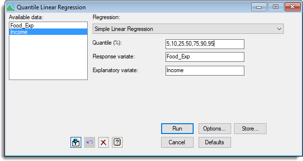
- Fill in the fields as shown below to fit a quantile simple linear regression to the relationship between household food expenditure (Food_Exp) and household income (Income) (both in Francs).
- Click Options to open the Options dialog and deselect Wald statistics then set Bootstrap method to None.
- Click OK to close the Options dialog then click Run.
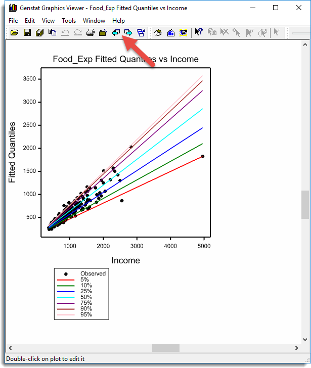
Running this regression produces a series of graphs including this one. Use the Next and Previous arrow buttons to step through the graphs.
Example 2
- Now close all windows and dialog and clear the data – from the menu select Data | Clear All Data and select Yes when prompted.
- From the menu select File | Open then navigate to the Windows default installation folder C:\Program Files\GenXXEd\Examples and select MelbourneTemp.gsh.
- From the menu select Stats | Regression Analysis | Quantile Regression.
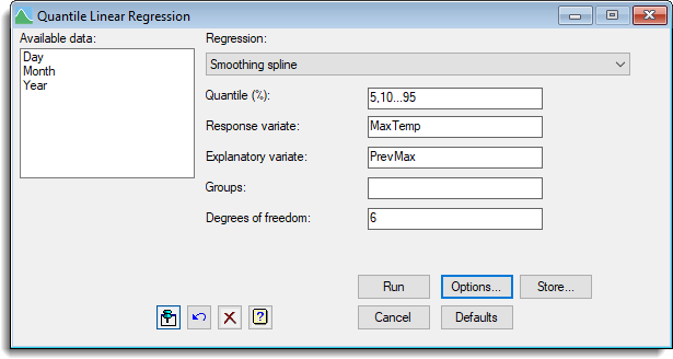
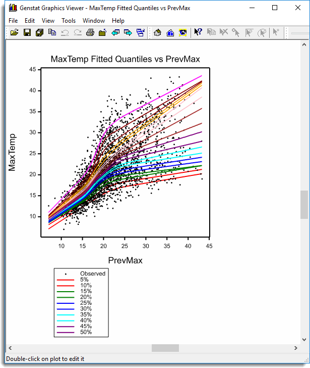
- Fill in the fields as shown below to it a spline with 6 d.f. to the relationship between today’s Maximum temperature (MaxTemp) and the previous day’s maximum temperature (PrevMax).
- Click Options to open the Options dialog and ensure Bootstrap method is set to None.
- Click OK to close the Options dialog then click Run.
Running this regression produces a series of graphs including this one. Use the Next and Previous arrow buttons to step through the graphs.
Action Icons
| Pin | Controls whether to keep the dialog open when you click Run. When the pin is down |
|
| Restore | Restore names into edit fields and default settings. | |
| Clear | Clear all fields and list boxes. | |
| Help | Open the Help topic for this dialog. |
See also
- Quantile Regression Options dialog
- Quantile Regression Store Options dialog
- Quantile Loess/Spline Regression Store Options dialog
- Nonlinear Quantile Regression menu
- Standard Curves menu
- Linear Regression menu
- Functional Linear Regression menu
- Simple Linear Regression menu
- Simple Linear Regression (with Groups) menu
- Multiple Linear Regression menu
- Multiple Linear Regression (with Groups) menu
- General Linear Regression menu
- Polynomial Regression menu
- Smoothing Spline menu
- Locally Weighted Regression menu
- Validation of Predictions menu.
- Circular Regression menu
- RQLINEAR procedure
- RQSMOOTH procedure
- FRQUANTILES directive
- RQNONLINEAR procedure
- RQOBJECTIVE function
- FIT directive for regression
- MINIMIZE procedure
- SIMPLEX procedure