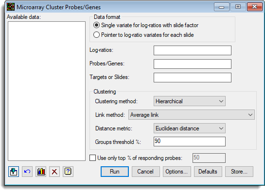
Select menu: Stats | Microarrays | Cluster | Probes/Genes
Use this to cluster probes (which may be thought of as representing genes) together on the similarity of their responses over a number of slides or target effects.
- After you have imported your data, from the menu select
Stats | Microarrays | Cluster | Probes/Genes. - Fill in the fields as required then click Run.
You can set additional Options before running and store the results by clicking Store.
The clustering may be either hierarchical or non-hierarchical using the k-means algorithm. A range of clustering criteria are available for each method. The probes are grouped together so that the responses of each group are similar, with the groups as distinct as possible. For the hierarchical clustering, the allocation to groups is specified by providing a threshold for the levels of similarity within a group, and the dendrogram is cut at this level generating an unknown number of groups. For the k-means algorithm, the number of groups must be specified.
A dendrogram for the hierarchical cluster analyses may be plotted, but for a large number of probes this is less useful as individual probes cannot be read. The responses of each probe across the targets/slides can also be plotted in a shade plot, but for large numbers of probes this is slow, in which case the mean response for each group can be plotted. A spreadsheet containing the grouped data can also be generated using the Store button.
With large numbers of probes, the limit of RAM can be quickly reached, so an option to only cluster probes with the largest mean absolute response is available.
Available data
This lists data structures appropriate for the field which currently has focus. Double-click a name to move it into the currently selected field or type the name in directly.
Data format
The data can be supplied in either of the following formats:
- Single variate for log-ratios with slide factor – All the log-ratios are stacked into a single variate, with factors that index the slide and probe/gene
- Pointer to log-ratio variates for each slide – Each slide has its data in a variate, and a pointer which points to this set of variates is provided. The Slides factor is not required, but if given should just have one entry for each slide in the order of the variates in the pointer. The Probes/Genes factor is that for a single slide, and all slides must have a common layout.
The spreadsheet stack and unstack menus can be used to reorganise the data between these two formats.
Log-ratios
The log-ratios to cluster the probes on.
Probes/Genes
The factor that identifies the probes or genes on a slide. If the data are in pointer format, this has just one entry per probe, but if the data are in variate (stacked) format, this factor indexes the probes in the log-ratio variate.
Targets or slides
The factor that identifies the slides. If the data are in pointer format, this has just one entry per slide, but if the data are in variate (stacked) format, this factor indexes the slides in the log-ratio variate.
Clustering method
The type of clustering to be used:
| Hierarchical | Hierarchical clustering using the method selected within the Link method option. |
| K-means | Non-hierarchical clustering using k-means method |
When a clustering method is selected the options and controls change to allow you to specify settings for the chosen method.
Link method (Hierarchical only)
A number of methods for clustering are available and vary according to the way in which ‘closest’ is defined at each stage of merging groups. The following possibilities are available:
| Single link | Defines the similarity between two clusters as the maximum similarity between any two samples in those clusters |
| Nearest neighbour | Synonym for Single link |
| Complete link | Defines the similarity between two clusters as the minimum similarity between any two samples in those clusters |
| Furthest neighbour | Synonym for Complete link |
| Average link | Defines the similarity between a cluster and two merging clusters as the average of the similarities with each of the original clusters. It therefore replaces two merging clusters by their mean, unweighted by cluster size |
| Group average | An average is taken over all the samples in the two merging clusters. Thus, the original clusters are replaced by their mean, weighted by cluster size |
| Median sorting | Can be thought of in terms of clusters being represented by points in a multidimensional space; when two clusters join, the new cluster is represented by the midpoint of the original cluster points |
Distance metric (Hierarchical only)
The method of combining the probe similarities.
| Type | Contribution |
| Euclidean | 1 – {(xi – xj) / range}**2 |
| Cityblock | 1 – |xi – xj| / range 1 |
Groups threshold% (Hierarchical only)
The minimum percentage similarity within groups. This is equivalent to drawing a line across the dendrogram and cutting it into the groups than have been joined below this threshold.
Criterion (K-means only)
The criterion to be optimized by the clustering. This can be set to one of the following four choices:
| Within-class dispersion | Minimizes the determinant of the pooled within-class dispersion matrix (W). Under the assumption that the data originated from a mixture of k multivariate Normal distributions, with equal variance-covariance matrix V, the MLE of V is obtained when the grouping into k classes minimizes det(W). Obtains compact groups. |
| Mahalanobis squared distance | Maximizes the total between-groups Mahalanobis squared distance. This will obtain separation of groups, possibly at the cost of compactness. Equivalent to the Within-class dispersion criterion when there are only two groups. |
| Between-group sum of squares | Minimizes the trace of the pooled within-class dispersion matrix (W). Equivalent to maximizing the total between-group sum of squares, or Euclidean distance between groups. |
| Maximal predictive classification | Maximal predictive classification is suitable for binary data. Each group has a class predictor, a binary indicator for each variate set to 0 or 1 according to whichever value is more frequent in the group. The criterion to be maximized is the total number of agreements between units and their respective class predictors. |
Number of probe groups (K-means only)
The number of clusters to group the probes into.
Use only top % of responding probes
Cluster only the a percentage of the probes. These probes chosen will be those with largest average absolute responses.
Action buttons
| Run | Run the analysis. |
| Cancel | Close the dialog without further changes. |
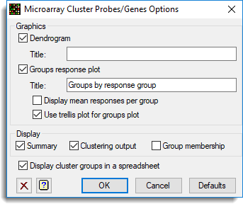
| Options | Opens a dialog where additional options and settings can be specified for the analysis. |
| Defaults | Reset the options back to their default settings. Clicking the right mouse on this button produces a pop-up menu where you can choose to set the options using the currently stored defaults or the Genstat default settings. |
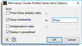
| Store | Opens a dialog to specify names of structures to store the results from the analysis. The names to save the structures must be supplied before running the analysis. |
Action Icons
| Pin | Controls whether to keep the dialog open when you click Run. When the pin is up |
|
| Restore | Restore names into edit fields and default settings. | |
| Graphics Output | Controls how graphs are to be drawn. You can either draw the graph in the Graphics View or save direct to files (JPEG, TIFF, EPS, EMF, GMF, BMP or PNG). | |
| Clear | Clear all fields and list boxes. | |
| Help | Open the Help topic for this dialog. |
Example
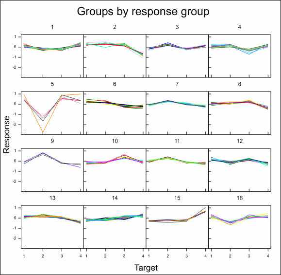
The following image shows the k-means clustering of a series of slides from a microarray experiment (Test_Slides_Estimates.gsh):
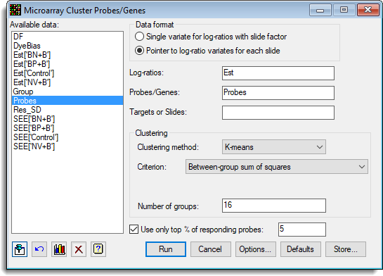
The options used were:
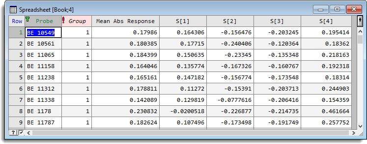
and the Store button as used to save Group results back to a spreadsheet:
The resulting response for each group is show below (by individual EST):
The spreadsheet generated by the Display in spreadsheet option is shown:
See also
- Cluster Probes/Genes Options
- Cluster Probes/Genes Store Options
- Cluster Targets/Slides
- Two-way Clustering
- Microarray Menus
- Two Channel Microarray Example
- Histograms, density plots, spatial plots and 2D plots for visualizing microarray data
- Volcano Plot
- Hierarchical Cluster Analysis
- Non-Hierarchical Cluster Analysis
- Microarray procedures
- MAPCLUSTER procedure
- HCLUSTER directive for hierarchical clustering
- CLUSTER directive for non-hierarchical clustering